# epydemix WebAPI — full documentation
Concatenated from the docs site. See https://epydemix-webapi.vercel.app/docs for the rendered version with navigation.
---
# AI Integration
The API is built so AI tools can use it directly. Two options, depending on how you work:
- **[Chat](#chat)**: discuss the API or get help building requests in a regular chat conversation.
- **[MCP server](#connect-via-mcp)**: let your AI assistant call the API directly as native tools, with no copy-paste or manual request bodies.
## Chat
To get help from an AI assistant in a regular chat, paste one of these resources into the prompt so it has accurate, up-to-date context about the API:
- **OpenAPI spec** [`/openapi.json`](https://epyscenario-api.isi.it/api/v1/openapi.json): every endpoint with field types and example values, ideal when you want help **building requests**.
- **Docs summary** [`/llms.txt`](https://epydemix-webapi.vercel.app/llms.txt) (~30 lines): short index of every doc page, good for general questions.
- **Full docs** [`/llms-full.txt`](https://epydemix-webapi.vercel.app/llms-full.txt) (~30 KB): every doc page concatenated, ideal for grounding deeper questions or for RAG ingestion.
Example prompts (use the copy button on each block):
```text
Using the OpenAPI spec, build an example JSON request for the SIR compartmental model with the United_States demographic dataset over a 6-month time window. This is for a numerical modeling exercise; only the request body is needed.
Docs: https://epydemix-webapi.vercel.app/llms.txt
OpenAPI spec: https://epyscenario-api.isi.it/api/v1/openapi.json
```
```text
Using the docs provided, explain how the parameter_transforms field of this compartmental-model API works and show one minimal example request body for each method (balcan, scale, override).
Docs: https://epydemix-webapi.vercel.app/llms.txt
OpenAPI spec: https://epyscenario-api.isi.it/api/v1/openapi.json
```
```text
Using the OpenAPI spec, generate a Python script using `requests` that runs the SIR simulation and prints the peak value of the new infection transitions from the median trajectory.
This is a textbook SIR exercise on a synthetic demographic dataset.
Docs: https://epydemix-webapi.vercel.app/llms.txt
OpenAPI spec: https://epyscenario-api.isi.it/api/v1/openapi.json
```
:::tip Enable browsing
Make sure the assistant has **web browsing or URL-fetch tools enabled** before pasting these prompts. The prompts reference live URLs (the OpenAPI spec, `llms.txt`, etc.); without browsing, the assistant cannot fetch them and will **hallucinate** endpoint names, field types, and requests which does not actually exist.
:::
:::tip Safety filters
Some flagship models occasionally **flag conversations about epidemic models for safety reasons** and stop returning responses, even though the underlying work is a purely numerical, theoretical compartmental-model exercise. If this happens, framing it as in the examples above (theoretical/numerical work, textbook SIR / SEIR / SIS) could be effective. Switching to smaller models (e.g., Claude Sonnet 4, GPT-5.3 Instant) may also help.
:::
## Connect via MCP
Model Context Protocol (MCP) lets AI assistants call this API as native tools, with no copy-paste or manual request bodies. Once connected, you just ask in plain language and the assistant handles the rest.
The endpoint is:
```
https://epyscenario-api.isi.it/mcp
```
Claude Desktop needs a small bridge for remote MCP servers. Add to `claude_desktop_config.json`:
```json
{
"mcpServers": {
"epydemix-webapi": {
"command": "npx",
"args": ["-y", "mcp-remote", "https://epyscenario-api.isi.it/mcp"]
}
}
}
```
Add the server with the `claude mcp add` command:
```bash
claude mcp add --transport http epydemix-webapi https://epyscenario-api.isi.it/mcp
```
This registers the server at user scope (available in every Claude Code session). Use `--scope project` if you want it tracked in a project-local `.mcp.json` instead.
Add to `~/.codex/config.toml`:
```toml
[mcp_servers.epydemix-webapi]
command = "npx"
args = ["-y", "mcp-remote", "https://epyscenario-api.isi.it/mcp"]
```
Add to your Cursor MCP settings:
```json
{
"mcpServers": {
"epydemix-webapi": {
"url": "https://epyscenario-api.isi.it/mcp"
}
}
}
```
In [claude.ai](https://claude.ai), open **Settings → Connectors → Add custom connector** and fill in:
- **Name**: `epydemix-webapi`
- **Remote MCP server URL**: `https://epyscenario-api.isi.it/mcp`
Once connected, try asking the assistant something like:
```text
Run the SIR compartmental model with the United_States demographic dataset
and Balcan summer-peak seasonality (max_value = 1, min_value = 0.1,
max_date in mid-July), then summarize the resulting numerical trajectories.
```
The assistant will pick the right tool, send the request, and explain the response.
---
# Running the API Locally
## Prerequisites
- [uv](https://docs.astral.sh/uv/) or Docker
## With uv
```bash
git clone https://github.com/mu373/epydemix-webapi.git
cd epydemix-webapi
uv sync
uv run uvicorn app.main:app --reload
```
The API is now running at `http://localhost:8000`.
## With Docker Compose
```bash
docker compose up
```
For hot reload during development:
```bash
docker compose --profile dev up api-dev
```
## Check it's working
```bash
curl http://localhost:8000/api/v1/health
```
```json
{"status": "healthy", "version": "0.1.1", "epydemix_version": "1.0.0"}
```
Swagger UI is available at `http://localhost:8000/api/v1/docs`.
---
# Google Cloud Run
This page covers deploying the API to Cloud Run, including the settings that matter for
performance under concurrent load. The recommended settings were validated by load
testing: tuning request concurrency alone gave roughly a 13x throughput and 10x latency
improvement.
## Prerequisites
- The [gcloud CLI](https://cloud.google.com/sdk/docs/install) installed and authenticated (`gcloud auth login`).
- A GCP project with billing enabled.
- The required APIs enabled
```bash
gcloud services enable run.googleapis.com cloudbuild.googleapis.com \
artifactregistry.googleapis.com --project=YOUR_PROJECT
```
## Container port
The image listens on the port given by the `PORT` environment variable, falling back to
8000 elsewhere. Cloud Run sets `PORT` automatically (8080 by default), so the container
just works with no extra flag.
## Deploy from source
`--source` uploads the repo, builds the image with Cloud Build using the Dockerfile,
pushes it to Artifact Registry, then deploys. No local Docker is needed.
```bash
gcloud run deploy epydemix-api \
--source . \
--project=YOUR_PROJECT \
--region=us-east1 \
--cpu=2 --memory=2Gi \
--concurrency=2 \
--min-instances=1 --max-instances=20 \
--timeout=120 \
--allow-unauthenticated
```
On success it prints the service URL, for example
`https://epydemix-api-XXXXXXXXX.us-east1.run.app`.
## Performance tuning
The simulation endpoint is CPU-bound. One SIR simulation (Nsim=20) takes about 1.5s, and
each uvicorn worker runs one at a time. With 2 workers on 2 vCPUs, a single instance sustains about
1.3 simulations per second.
- **`--concurrency=2`** is the key setting and must match the worker and vCPU count. The
Cloud Run default is 80, which routes up to 80 simulations to one 2-worker instance.
They queue behind the workers and latency climbs to 30 to 60 seconds. Setting
concurrency to 2 means each instance only takes what it can run in parallel, so Cloud
Run scales out to more instances instead of overloading one.
- **`--cpu=2`** must agree with uvicorn `--workers 2`. More workers than vCPUs only
time-share the CPU and add no throughput.
- **`--max-instances=20`** sets the throughput ceiling: 20 instances times ~1.3/s is
about 26 simulations per second. Raise it if you need more.
- **`--min-instances=1`** keeps a warm instance so the first request avoids a cold start
(container boot, epydemix import, population cache warm). Set it higher before a known
spike such as a workshop.
- **`--timeout=120`** is the Cloud Run request timeout. The app also self-limits to 60s.
## Verify
```bash
URL=https://epydemix-api-XXXXXXXXX.us-east1.run.app
curl -s "$URL/api/v1/health"
```
A single SIR simulation (Nsim=20) should return HTTP 200 in about 1.5s.
## Cost management
`--min-instances=1` keeps a container running continuously, which bills around the clock.
When not actively serving, scale to zero or delete:
```bash
# scale to zero (keep the service, stop idle billing):
gcloud run services update epydemix-api --project=YOUR_PROJECT --region=us-east1 --min-instances=0
# delete entirely:
gcloud run services delete epydemix-api --project=YOUR_PROJECT --region=us-east1
```
## Redeploy a prebuilt image
To redeploy with changed settings without rebuilding, point at the existing image in
Artifact Registry:
```bash
gcloud run deploy epydemix-api \
--image us-east1-docker.pkg.dev/YOUR_PROJECT/cloud-run-source-deploy/epydemix-api:latest \
--project=YOUR_PROJECT --region=us-east1 \
--cpu=2 --memory=2Gi --concurrency=2 \
--min-instances=1 --max-instances=20 --timeout=120 --allow-unauthenticated
```
## Terraform
Terraform does not build images. Build and push first
(`gcloud builds submit --tag ...` or `docker push`), then reference the image:
```hcl
resource "google_cloud_run_v2_service" "api" {
name = "epydemix-api"
location = "us-east1"
template {
scaling {
min_instance_count = 1
max_instance_count = 20
}
max_instance_request_concurrency = 2 # the key knob
timeout = "120s"
containers {
image = "us-east1-docker.pkg.dev/YOUR_PROJECT/REPO/epydemix-api:latest"
resources {
limits = { cpu = "2", memory = "2Gi" }
}
}
}
}
```
---
# Production
## Fly.io
The project includes a `fly.toml` configuration. Make sure [flyctl](https://fly.io/docs/hands-on/install-flyctl/) is installed and you're logged in.
```bash
fly auth login
fly deploy
```
## Docker
Build and run the production image:
```bash
docker build -t epydemix-api .
docker run -p 8000:8000 epydemix-api
```
## Google Cloud Run
Deploy from source with Cloud Build:
```bash
gcloud run deploy epydemix-api --source . --region=us-east1 \
--cpu=2 --concurrency=2 --max-instances=20 --allow-unauthenticated
```
The simulation endpoint is CPU-bound, so set `--concurrency` to match the worker/vCPU
count, otherwise requests queue on an overloaded instance instead of scaling out. See
[Google Cloud Run](./google-cloud-run.md) for the full guide and tuning rationale.
## Environment variables
See [Configuration](/docs/reference/configuration) for all available settings.
---
# FAQ
## Models
### How do I define a custom model?
Skip `model.preset` and provide three fields under `model`: a list of `compartments`, a `parameters` dict, and a list of `transitions`. Each transition has a `source` compartment, a `target`, a `kind` (`spontaneous` or `mediated`), and `params` referencing entries from `parameters`.
```json
"model": {
"compartments": ["S", "E", "I", "R"],
"parameters": {
"transmission_rate": 0.3,
"incubation_rate": 0.2,
"recovery_rate": 0.1
},
"transitions": [
{"source": "S", "target": "E", "kind": "mediated", "params": ["transmission_rate", "I"]},
{"source": "E", "target": "I", "kind": "spontaneous", "params": "incubation_rate"},
{"source": "I", "target": "R", "kind": "spontaneous", "params": "recovery_rate"}
]
}
```
See [Model › Custom Models](./guides/model/custom-models.mdx) for the full structure and a worked SEIRH example.
### How do I make simulations reproducible?
Pass an integer `seed` under `simulation`. The same request with the same seed returns identical trajectories.
```json
"simulation": {
"start_date": "2024-01-01",
"end_date": "2024-06-01",
"Nsim": 10,
"seed": 42
}
```
## Parameters
### How do I set a rate instead of a period for a transition?
Preset disease-history parameters accept either a period (in days) or its corresponding rate (per day). Pass whichever form is more convenient and the resolver injects the other automatically as `rate = 1 / period`.
| Period (days) | Rate (1/day) |
|---|---|
| `incubation_period` | `incubation_rate` |
| `infectious_period` | `recovery_rate` |
| `hosp_duration` | `hosp_recovery_rate` |
| `immunity_duration` | `waning_rate` |
For example, to set the recovery rate directly instead of the infectious period:
```json
"parameters": {
"R0": 2.5,
"incubation_period": 3.0,
"recovery_rate": 0.4
}
```
Pass *either* the period or the rate, not both. If both are sent the rate form wins and the period is dropped silently. Conversions are preset-scoped; see each preset's Parameters table for which conversions it accepts.
### How do I set the transmission rate directly instead of R0?
`R0` and `transmission_rate` are parameters for transmission, and are associated with each other. By default, the preset takes `R0` and derives `transmission_rate` from it via a preset-specific formula, which depends on the next-generation matrix of the model's infectious compartments. You can also directly set `transmission_rate` to bypass the conversion.
```json
"parameters": {
"transmission_rate": 0.4,
}
```
If both are sent, `transmission_rate` wins and `R0` is dropped silently. See each preset's Parameters table for the conversion formula it uses, and [Model › Parameters › Calculated parameters](./guides/model/parameters/overview.mdx#calculated-parameters) for the resolver machinery.
### How do I make a parameter age-varying?
Pass a list under `model.parameters` instead of a scalar. The list length must equal the number of resolved age groups (after `age_group_mapping` is applied).
```json
"parameters": {
"transmission_rate": [0.35, 0.35, 0.30, 0.25, 0.20]
}
```
See [Model › Parameters](./guides/model/parameters/overview.mdx#age-varying-parameters).
### How do I apply seasonality?
Add `parameter_transforms` with `balcan` method targeting the parameter you want to modulate. Set `max_date` / `min_date` to the seasonal peak / trough and `max_value` / `min_value` to the bounds. The existing parameter value is multiplied by a sinusoidal factor in `[min_value/max_value, 1]`.
```json
"parameter_transforms": [
{
"target_parameter": "transmission_rate",
"method": "balcan",
"max_date": "2024-01-15",
"min_date": "2024-07-15",
"max_value": 1,
"min_value": 0.1
}
]
```
See [Parameter Transforms › Seasonality](./guides/model/parameters/transformations.mdx#seasonality) for the math.
### How do I override a parameter for a date range?
Use a `parameter_transforms` entry with `method: "override"`. The replacement is absolute (not multiplicative) and always wins for its window. Pass a scalar or a per-age-group list as `value`.
```json
"parameter_transforms": [
{
"target_parameter": "transmission_rate",
"method": "override",
"start_date": "2024-03-01",
"end_date": "2024-04-01",
"value": 0.05
}
]
```
See [Parameter Transforms › Override](./guides/model/parameters/transformations.mdx#override).
### What's the difference between `scale` and `override`?
| | `scale` | `override` |
|---|---|---|
| Operation | Multiplicative (`baseline × factor`) | Absolute replacement (ignores baseline) |
| Composition | Stacks with other `scale` and `balcan` transforms | Always wins for its date window |
| Outside window | Multiplier is 1.0 (no change) | Original baseline applies |
Use `scale` when you want a relative change (e.g. "halve transmission during this window") and `override` when you want a known absolute value (e.g. "set transmission to exactly 0.05 during this window").
### How do I see the effective parameter values?
Set `output.include_parameters: true`. The response gains a `results.parameters` section with per-step values for every model parameter, broadcast to per-age-group arrays. Override windows are baked in, so the array reflects what actually drove the simulation.
```json
"output": { "include_parameters": true }
```
See [Parameter Transforms › Inspecting the effective parameter values](./guides/model/parameters/transformations.mdx#inspecting-the-effective-parameter-values).
## Vaccination
### How do I disable vaccination rollout in a V-SEIHR run?
Omit the `vaccination` block entirely from the request. The `Susceptible → Susceptible_vax` flow is added only when `vaccination` is present; without it the vaccinated branch stays at zero for the whole run and V-SEIHR behaves like plain SEIHR.
An empty `"vaccination": {"campaigns": []}` is rejected as a 422 (`vaccination.campaigns must contain at least one entry`), so just leave the block out instead. See [V-SEIHR › Without vaccination](./guides/model/presets/v-seihr.mdx#without-vaccination) for a full request example.
---
# Initial Conditions
The `initial_conditions` block seeds the model's compartments at the start of the simulation. Two methods are supported: `percentage` (default) and `absolute`. If you omit the block entirely, [epydemix's built-in default](#default-when-omitted) is used.
## `percentage`
Specify the share of the population in each compartment as a **percentage** (not a fraction). The values are divided by 100 internally, distributed proportionally across age groups, and whatever is left over goes to the first compartment of the preset (usually `Susceptible`).
| Field | Type | Notes |
|---|---|---|
| `method` | `"percentage"` | Default. |
| `initial_percentages` | `{compartment: number}` | Percentages of total population. `0.1` = 0.1%, `10.0` = 10%. |
### Example: seed 0.1% as infected
```bash
curl -X POST BASE_URL/simulations \\
-H "Content-Type: application/json" \\
-d '{
"model": {
"preset": "SIR",
"parameters": {"R0": 2.5, "infectious_period": 10.0}
},
"population": {"name": "United_States"},
"simulation": {"start_date": "2024-01-01", "end_date": "2024-04-01", "Nsim": 10},
"initial_conditions": {
"method": "percentage",
"initial_percentages": {"Infected": 0.1}
}
}'
```
### Example: seed multiple compartments
The remainder (after `Infected` and `Recovered`) lands in `Susceptible`. Here 1% infected, 30% already recovered (e.g. modeling a population with prior immunity), and 69% susceptible.
```bash
curl -X POST BASE_URL/simulations \\
-H "Content-Type: application/json" \\
-d '{
"model": {
"preset": "SIR",
"parameters": {"R0": 2.5, "infectious_period": 10.0}
},
"population": {"name": "United_States"},
"simulation": {"start_date": "2024-01-01", "end_date": "2024-04-01", "Nsim": 10},
"initial_conditions": {
"method": "percentage",
"initial_percentages": {"Infected": 1.0, "Recovered": 30.0}
}
}'
```
The percentage of each compartment is split across age groups in proportion to each group's share of the total population, so larger age groups receive proportionally more seed counts.
## `absolute`
Specify exact counts per compartment per age group. You are responsible for making the counts sum to the population in each age group; nothing is auto-filled.
| Field | Type | Notes |
|---|---|---|
| `method` | `"absolute"` | |
| `compartments` | `{compartment: number[]}` | One array per compartment. Array length must equal the population's number of age groups. |
### Example: explicit per-age counts
The five-bin default for `United_States` has age groups `[0-19, 20-49, 50-64, 65-74, 75+]`. The arrays below seed 100 / 200 / 500 / 500 / 200 infected per age group; the rest of each group sits in `Susceptible`.
```bash
curl -X POST BASE_URL/simulations \\
-H "Content-Type: application/json" \\
-d '{
"model": {
"preset": "SIR",
"parameters": {"R0": 2.5, "infectious_period": 10.0}
},
"population": {"name": "United_States"},
"simulation": {"start_date": "2024-01-01", "end_date": "2024-04-01", "Nsim": 10},
"initial_conditions": {
"method": "absolute",
"compartments": {
"Susceptible": [83000000, 132000000, 62000000, 32000000, 22000000],
"Infected": [100, 200, 500, 500, 200]
}
}
}'
```
If the array length doesn't match the population's age groups, the request is rejected.
## Default when omitted
If you omit `initial_conditions`, ~0.05% of each age group is seeded into `Infected` and the rest into `Susceptible`. For V-SEIHR, the `_vax` branch starts at zero.
## Notes
- Compartment names in `initial_percentages` / `compartments` must match the preset's compartment names (e.g. `Susceptible`, `Exposed`, `Infected`, `Recovered`, `Hospitalized` for SEIHR-family presets; `_vax` twins for V-SEIHR).
- For V-SEIHR, the vaccinated branch (`Susceptible_vax`, `Exposed_vax`, …) starts at zero unless you seed it or supply a [`vaccination`](./vaccination/overview.mdx) block.
- Use [Custom Models](./model/custom-models.mdx) if you need compartments outside the preset list.
---
# Custom Models
Instead of using a preset, you can define your own compartmental model by specifying compartments, parameters, and transitions. See the [API Reference](/api-reference) for the full request schema.
## Model structure
A custom model requires three things: `compartments`, `parameters`, and `transitions`.
### Compartments
A list of states that individuals can be in. The first compartment is treated as the default state for the remaining population when setting initial conditions.
```json
"compartments": ["S", "E", "I", "R", "H"]
```
### Parameters
Named rate values referenced by transitions. Each key is a parameter name and the value is its rate. All parameters used in transitions must be defined here.
```json
"parameters": {
"transmission_rate": 0.3,
"recovery_rate": 0.1,
"incubation_rate": 0.2,
"hospitalization_rate": 0.05,
"recovery_rate_h": 0.15
}
```
### Transitions
Rules for how individuals move between compartments. Each transition has a `source`, `target`, `kind`, and `params`. The `source` and `target` must match compartment names defined above.
There are two kinds:
- **Spontaneous**: occurs at a fixed rate, independent of other compartments. `params` is a single parameter name.
- **Mediated**: rate depends on the proportion of individuals in another compartment. `params` is a two-element list `[rate_parameter, mediating_compartment]`.
Examples:
```json
"transitions": [
{"source": "I", "target": "R", "kind": "spontaneous", "params": "recovery_rate"},
{"source": "S", "target": "E", "kind": "mediated", "params": ["transmission_rate", "I"]}
]
```
## Example: SEIRH model
This model extends SEIR with a hospitalized compartment. Infected individuals may either recover directly or be hospitalized first. The example below seeds 0.1% of the population as `I` at t=0 via an explicit `initial_conditions` block; the rest starts in `S`. See [Initial Conditions](../initial-conditions.mdx) for other seeding options. Custom models have no built-in default. If you omit the block, epydemix's fallback is used, but it can misspecify the initial state for some model structures.
```bash
curl -X POST BASE_URL/simulations \\
-H "Content-Type: application/json" \\
-d '{
"model": {
"compartments": ["S", "E", "I", "R", "H"],
"parameters": {
"transmission_rate": 0.3,
"incubation_rate": 0.2,
"recovery_rate": 0.1,
"hospitalization_rate": 0.05,
"recovery_rate_h": 0.15
},
"transitions": [
{"source": "S", "target": "E", "kind": "mediated", "params": ["transmission_rate", "I"]},
{"source": "E", "target": "I", "kind": "spontaneous", "params": "incubation_rate"},
{"source": "I", "target": "H", "kind": "spontaneous", "params": "hospitalization_rate"},
{"source": "I", "target": "R", "kind": "spontaneous", "params": "recovery_rate"},
{"source": "H", "target": "R", "kind": "spontaneous", "params": "recovery_rate_h"}
]
},
"population": {"name": "United_States"},
"simulation": {
"start_date": "2024-01-01",
"end_date": "2024-03-01",
"Nsim": 10
},
"initial_conditions": {
"method": "percentage",
"initial_percentages": {"I": 0.1}
}
}'
```
### Transitions breakdown
| Source | Target | Kind | Parameter |
|---|---|---|---|
| S | E | mediated | `transmission_rate`, mediated by I |
| E | I | spontaneous | `incubation_rate` |
| I | H | spontaneous | `hospitalization_rate` |
| I | R | spontaneous | `recovery_rate` |
| H | R | spontaneous | `recovery_rate_h` |
---
# Overview
Parameters are the named rate values referenced by your model's transitions. Every parameter used in a [preset](../presets/overview.mdx) or [custom model](../custom-models.mdx) transition must appear under `model.parameters`. Three value shapes are supported: scalar, age-varying, and calculated (expressions over other parameters).
## Scalar parameters
A single rate that applies uniformly to every age group. This is the default.
```bash
curl -X POST BASE_URL/simulations \\
-H "Content-Type: application/json" \\
-d '{
"model": {
"preset": "SIR",
"parameters": {
"transmission_rate": 0.3,
"recovery_rate": 0.1
}
},
"population": { "name": "United_States" },
"simulation": {
"start_date": "2024-01-01",
"end_date": "2024-06-01",
"Nsim": 10
}
}'
```
## Age-varying parameters
A list of one rate per age group. The list length must match the number of age groups in the resolved population (after any `age_group_mapping` is applied).
For example, with the 5-group mapping below, `transmission_rate = [0.35, 0.35, 0.30, 0.25, 0.20]` means the youngest two groups transmit at 0.35, the middle group at 0.30, and so on.
```bash
curl -X POST BASE_URL/simulations \\
-H "Content-Type: application/json" \\
-d '{
"model": {
"preset": "SIR",
"parameters": {
"transmission_rate": [0.35, 0.35, 0.30, 0.25, 0.20],
"recovery_rate": [0.10, 0.10, 0.10, 0.08, 0.06]
}
},
"population": {
"name": "United_States",
"contacts_source": "prem_2021",
"age_group_mapping": {
"0-4": ["0-4"],
"5-17": ["5-9", "10-14", "15-19"],
"18-49": ["20-24", "25-29", "30-34", "35-39", "40-44", "45-49"],
"50-64": ["50-54", "55-59", "60-64"],
"65+": ["65-69", "70-74", "75+"]
}
},
"simulation": {
"start_date": "2024-01-01",
"end_date": "2024-12-31",
"Nsim": 10
}
}'
```
You can mix scalar and age-varying values across parameters. For example, `transmission_rate` can be age-varying while `recovery_rate` stays scalar.
## Calculated parameters
A string value in `parameters` is treated as an arithmetic expression over the **other** parameters. The expression is evaluated at simulation build time and the result is stored under that name like any other parameter. Useful for branching outflow rates (e.g. `(1 - p_h) * gamma`) and for deriving one parameter from another (e.g. `transmission_rate` from a target $R_0$).
```json
{
"parameters": {
"p_h": 0.05,
"gamma": 0.1,
"alpha": 0.2,
"recovery_rate": "(1 - p_h) * gamma",
"hospitalization_rate": "p_h * alpha"
}
}
```
Source-parameter shapes propagate via numpy broadcasting. If `p_h` is age-varying (`[0.05, 0.10, 0.15, 0.20, 0.25]`), then `(1 - p_h) * gamma` is automatically age-varying too. If `gamma` is also seasonally scaled via [`parameter_transforms`](./transformations.mdx), the calculated parameter inherits the time-variation as well — calculated parameters evaluate **after** transforms.
### Allowed expression syntax
Strict arithmetic only:
- Binary operators: `+`, `-`, `*`, `/`, `//`, `**`, `%`
- Unary operators: `+`, `-`
- Parentheses for grouping
- Numeric literals
- Names of other parameters (or reserved names below)
Function calls, attribute access, subscripts, comparisons, and conditionals are rejected with a `422` error. This keeps expressions safe to evaluate and easy to read.
### Transforms on calculated parameters
A calculated parameter **can** be the `target_parameter` of a [`parameter_transform`](./transformations.mdx). The transform layers on top of the evaluated expression: source-targeted transforms run first, then expressions are evaluated (so the sources' post-transform values feed in), then any transform targeting a calc-param applies to the result. Use this when you want to modulate a derived parameter directly without changing every source it depends on, e.g. a flat scale on `transmission_rate_vax` while a `balcan` envelope modulates `transmission_rate`.
### Restrictions
- Circular dependencies among expressions (`a = "b + 1", b = "a + 1"`) are rejected with a `422`.
- A reference to an undefined name is rejected with a `422` naming the missing parameter.
### Reserved names
Expressions can also reference SCREAMING_SNAKE_CASE constants derived from the model state. User parameters cannot share these names.
| Name | Value |
|---|---|
| `CONTACT_MATRIX_EIGENVALUE_ALL` | Dominant eigenvalue (largest by magnitude) of the sum of all contact-matrix layers in the resolved population. |
The most common use is calibrating `transmission_rate` from a target $R_0$:
```bash
curl -X POST BASE_URL/simulations \\
-H "Content-Type: application/json" \\
-d '{
"model": {
"preset": "SIR",
"parameters": {
"R0": 1.5,
"gamma": 0.1,
"recovery_rate": "gamma",
"transmission_rate": "R0 * gamma / CONTACT_MATRIX_EIGENVALUE_ALL"
}
},
"population": { "name": "United_States" },
"simulation": {
"start_date": "2024-01-01",
"end_date": "2024-06-01",
"Nsim": 10
}
}'
```
Reserved names exist only in the expression namespace; they are not stored on the model and so do not appear under `results.parameters`.
## Time-varying parameters
To make parameters change over the course of the simulation (seasonality, scaling windows, or absolute overrides), use [`parameter_transforms`](./transformations.mdx). Transforms compose on top of whatever you set here, so a base scalar or age-varying parameter still acts as the starting point.
---
# Transformations
`parameter_transforms` lets you modify model parameters during a simulation. Use them to apply seasonality, scale a parameter during a window, or replace it outright. Three methods are supported:
| Method | What it does | Applied when |
|---|---|---|
| `balcan` | Sinusoidal seasonality across the whole simulation timeline (multiplicative) | pre-simulation |
| `scale` | Constant multiplicative factor over a date window | pre-simulation |
| `override` | Absolute replacement value over a date window (scalar or per age group) | during simulation |
All three transforms target an existing parameter via `target_parameter`, which must already be defined in `model.parameters`. Both source parameters (scalar or age-varying) and [calculated parameters](./overview.mdx#calculated-parameters) are valid targets. Transforms on a source propagate through any expression that references it; transforms on a calc-param itself apply *after* the expression is evaluated, so the two compose naturally (see [Transforms on calculated parameters](./overview.mdx#transforms-on-calculated-parameters)).
## Composition order
Multiple transforms on the same parameter compose:
- `balcan` and `scale` stack **multiplicatively** in the order you list them. `[balcan, scale(0.5)]` first applies the seasonal envelope, then halves it.
- `override` always wins for its date window, regardless of where it appears in the list (epydemix stores overrides separately from `model.parameters`).
## Seasonality
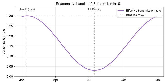
Sinusoidal seasonality based on Balcan D et al., *J. Comput. Sci.* 2010 ([DOI: 10.1016/j.jocs.2010.07.002](https://doi.org/10.1016/j.jocs.2010.07.002), eq. 25). The transform is **multiplicative on top of the baseline parameter**: at each step, the existing value is multiplied by a sinusoidal factor that reaches `1.0` on `max_date` (the seasonal peak) and `min_value / max_value` on `min_date` (the seasonal trough). The effective parameter therefore swings between `baseline` (peak) and `baseline × (min_value / max_value)` (trough).
**Recommended usage**: leave `max_value` at its default of `1.0` and only set `min_value` to express the seasonal floor as a fraction of the baseline. For example, `min_value=0.1` means "the parameter drops to 10% of baseline at the trough."
The seasonal factor at time $t$ (days since the simulation start) is
$$
s(t) = \frac{1}{2} \left[ \left(1 - \frac{v_{\min}}{v_{\max}}\right) \sin\!\left(\frac{2\pi}{T}\,(t - t_{\max}) + \frac{\pi}{2}\right) + 1 + \frac{v_{\min}}{v_{\max}} \right],
$$
where:
- $v_{\min}$, $v_{\max}$: `min_value` and `max_value`
- $t_{\max}$: day index of `max_date`
- $T$: period in days; `2 × |min_date − max_date|` if `min_date` is set, otherwise 365
The effective parameter is then `baseline × s(t)`, ranging in `[baseline × min_value/max_value, baseline]`.
For example, with `transmission_rate = 0.3`, `min_value = 0.1`, `max_date = 2024-01-15`, and `min_date = 2024-07-15` (and the default `max_value = 1`), the effective rate is `0.3 × 1 = 0.3` on Jan 15 and `0.3 × 0.1 = 0.03` on Jul 15, sweeping smoothly between the two over the year.
| Field | Required | Description |
|---|---|---|
| `target_parameter` | yes | Parameter name to modulate (e.g. `transmission_rate`). |
| `max_date` | yes | Date when the multiplier reaches its peak (1.0), `YYYY-MM-DD`. |
| `min_value` | yes | Lower bound of the seasonal scaling. With the default `max_value=1`, this is the fraction of baseline at the trough (e.g. `0.1` = 10% of baseline). |
| `max_value` | no | Upper bound of the seasonal scaling. Defaults to `1.0`. Only set this if you want to express both bounds in absolute units; only the **ratio** `min_value / max_value` affects the dynamics. |
| `min_date` | no | Date of the trough. If set, period = `2 × |min_date − max_date|`. If omitted, period = 365 days. |
```bash
curl -X POST BASE_URL/simulations \\
-H "Content-Type: application/json" \\
-d '{
"model": {
"preset": "SIR",
"parameters": { "transmission_rate": 0.3, "recovery_rate": 0.1 }
},
"population": { "name": "United_States" },
"simulation": {
"start_date": "2024-01-01",
"end_date": "2024-12-31",
"Nsim": 50,
"seed": 42
},
"parameter_transforms": [
{
"target_parameter": "transmission_rate",
"method": "balcan",
"max_date": "2024-01-15",
"min_date": "2024-07-15",
"min_value": 0.1
}
]
}'
```
## Scale
Multiply a parameter by a constant `factor` inside `[start_date, end_date]`; outside the window the multiplier is 1.0.
For example, if `transmission_rate = 0.1` and `factor = 0.5`, the effective rate is `0.1 × 0.5 = 0.05` inside the window, and `0.1` everywhere else.
![Scale example: baseline 0.1 with factor 0.5 inside [Mar 1, Apr 1]](/img/parameter-transforms/scale.svg)
| Field | Required | Description |
|---|---|---|
| `target_parameter` | yes | Parameter name to scale. |
| `start_date` | yes | Window start, `YYYY-MM-DD`. |
| `end_date` | yes | Window end, `YYYY-MM-DD`. Must be `≥ start_date`. |
| `factor` | yes | Multiplicative factor applied within the window. |
```bash
curl -X POST BASE_URL/simulations \\
-H "Content-Type: application/json" \\
-d '{
"model": { "preset": "SIR" },
"population": { "name": "United_States" },
"simulation": {
"start_date": "2024-01-01",
"end_date": "2024-06-01",
"Nsim": 10
},
"parameter_transforms": [
{
"target_parameter": "transmission_rate",
"method": "scale",
"start_date": "2024-03-01",
"end_date": "2024-04-01",
"factor": 0.5
}
]
}'
```
## Override
Replace a parameter outright during a date window. The replacement can be a scalar or a per-age-group list (length must match the resolved population's age groups).
For example, if `transmission_rate = 0.3` and an override sets `value = 0.1` for `[2024-03-01, 2024-04-01]`, the rate is `0.1` everywhere inside that window and `0.3` outside, irrespective of any `balcan` or `scale` transforms also targeting the same parameter.
![Override example: baseline 0.3 with value 0.1 inside [Mar 1, Apr 1]](/img/parameter-transforms/override.svg)
| Field | Required | Description |
|---|---|---|
| `target_parameter` | yes | Parameter name to override. |
| `start_date` | yes | Window start, `YYYY-MM-DD`. |
| `end_date` | yes | Window end, `YYYY-MM-DD`. Must be `≥ start_date`. |
| `value` | yes | Scalar (`float`) or per-age-group list (`list[float]`). |
### Scalar override
```bash
curl -X POST BASE_URL/simulations \\
-H "Content-Type: application/json" \\
-d '{
"model": { "preset": "SIR" },
"population": { "name": "United_States" },
"simulation": {
"start_date": "2024-01-01",
"end_date": "2024-06-01",
"Nsim": 10
},
"parameter_transforms": [
{
"target_parameter": "transmission_rate",
"method": "override",
"start_date": "2024-03-01",
"end_date": "2024-04-01",
"value": 0.1
}
]
}'
```
### Per-age-group override
The list length must equal the number of age groups in your resolved population.
```bash
curl -X POST BASE_URL/simulations \\
-H "Content-Type: application/json" \\
-d '{
"model": { "preset": "SIR" },
"population": {
"name": "United_States",
"contacts_source": "prem_2021",
"age_group_mapping": {
"0-4": ["0-4"],
"5-17": ["5-9", "10-14", "15-19"],
"18-49": ["20-24", "25-29", "30-34", "35-39", "40-44", "45-49"],
"50-64": ["50-54", "55-59", "60-64"],
"65+": ["65-69", "70-74", "75+"]
}
},
"simulation": {
"start_date": "2024-01-01",
"end_date": "2024-06-01",
"Nsim": 10
},
"parameter_transforms": [
{
"target_parameter": "transmission_rate",
"method": "override",
"start_date": "2024-03-01",
"end_date": "2024-04-01",
"value": [0.10, 0.12, 0.10, 0.08, 0.06]
}
]
}'
```
## Inspecting the effective parameter values
To verify what actually drove the simulation (handy for plotting seasonality curves or sanity-checking overrides), set `output.include_parameters: true`. The response gains a `results.parameters` section with the per-step value of every model parameter, broadcast to per-age-group arrays. Override windows are baked in.
The `parameters` section is **shared across stochastic runs**: parameters are deterministic inputs, so there's a single array per parameter regardless of `Nsim`. Off by default to keep responses small.
```bash
curl -X POST BASE_URL/simulations \\
-H "Content-Type: application/json" \\
-d '{
"model": {
"preset": "SIR",
"parameters": { "transmission_rate": 0.3, "recovery_rate": 0.1 }
},
"population": { "name": "United_States" },
"simulation": {
"start_date": "2024-01-01",
"end_date": "2024-12-31",
"Nsim": 10
},
"parameter_transforms": [
{
"target_parameter": "transmission_rate",
"method": "balcan",
"max_date": "2024-01-15",
"min_date": "2024-07-15",
"max_value": 1,
"min_value": 0.1
}
],
"output": { "include_parameters": true }
}'
```
The relevant slice of the response:
```json
{
"results": {
"parameters": {
"dates": ["2024-01-01", "2024-01-02", "..."],
"data": {
"transmission_rate": {
"0-4": [0.296, 0.297, "..."],
"5-19": [0.296, 0.297, "..."],
"...": []
},
"recovery_rate": {
"0-4": [0.10, 0.10, "..."]
}
}
}
}
}
```
:::tip
Use the [API Reference](/api-reference) to explore each transform schema field-by-field and try requests interactively.
:::
---
# Overview
## What are model presets?
Model presets are built-in compartmental epidemic models that you can use without defining compartments or transitions yourself. Each preset comes with a set of compartments, default parameters, and transition rules.
You can list all available presets:
```bash
curl BASE_URL/models/presets
```
## Available presets
| Preset | Compartments | Use when |
|---|---|---|
| [SIR](./sir.mdx) | S, I, R | You want the simplest possible epidemic model with permanent immunity. |
| [SEIR](./seir.mdx) | S, E, I, R | You need a latent (exposed-but-not-yet-infectious) period before infectiousness. |
| [SIS](./sis.mdx) | S, I | Recovered individuals return to the susceptible pool with no lasting immunity (e.g. many bacterial infections). |
| [V-SEIHR](./v-seihr.mdx) | 10 (S/E/I/H/R × unvaccinated/vaccinated) | You want SEIR with explicit hospitalization, a vaccinated branch, and a vaccination rollout via [the `vaccination` block](../../vaccination/overview.mdx). |
If none of these fit, you can declare compartments and transitions yourself. See [Custom Models](../custom-models.mdx).
---
# SEIR
The Susceptible-Exposed-Infected-Recovered model. Extends SIR with an exposed (latent) period before individuals become infectious.
## Compartments
- **Susceptible**: individuals who can be infected
- **Exposed**: individuals who are infected but not yet infectious (latent period)
- **Infected**: individuals who are currently infectious
- **Recovered**: individuals who have recovered and are immune
## Transitions
- **Susceptible → Exposed**: mediated by `transmission_rate` and the number of Infected individuals
- **Exposed → Infected**: spontaneous at `incubation_rate`
- **Infected → Recovered**: spontaneous at `recovery_rate`
## Parameters
Some parameters can be provided in multiple forms. For example, you can pass `R0` instead of `transmission_rate`, `incubation_period` instead of `incubation_rate`, or `infectious_period` instead of `recovery_rate`, and they are automatically converted. If both forms are supplied, the rate form wins and the source is dropped silently. See [calculated parameters](../parameters/overview.mdx#reserved-names) for the conversion machinery.
| Parameter | Status | Default | Description |
|---|---|---|---|
| `transmission_rate` | Default | `0.3` | $\beta$. Per-contact transmission rate. |
| `R0` | Alternative to `transmission_rate` | unset | Basic reproduction number. When passed, `transmission_rate = R0 * recovery_rate / CONTACT_MATRIX_EIGENVALUE_ALL`. |
| `incubation_rate` | Default | `0.2` | E → I rate. |
| `incubation_period` | Alternative to `incubation_rate` | unset | Days from exposure to infectiousness. When passed, `incubation_rate = 1 / incubation_period`. |
| `recovery_rate` | Default | `0.1` | I → R rate. |
| `infectious_period` | Alternative to `recovery_rate` | unset | Days infectious. When passed, `recovery_rate = 1 / infectious_period`. |
## Examples
Both examples below seed 0.1% of the population as `Exposed` at t=0 via an explicit `initial_conditions` block; the rest of the population starts in `Susceptible`. See [Initial Conditions](../../initial-conditions.mdx) for other seeding options.
### Rate form
```bash
curl -X POST BASE_URL/simulations \\
-H "Content-Type: application/json" \\
-d '{
"model": {
"preset": "SEIR",
"parameters": {"transmission_rate": 0.3, "incubation_rate": 0.2, "recovery_rate": 0.1}
},
"population": {"name": "United_States"},
"simulation": {"start_date": "2024-01-01", "end_date": "2024-06-01", "Nsim": 10},
"initial_conditions": {
"method": "percentage",
"initial_percentages": {"Exposed": 0.1}
}
}'
```
### Using `R0` and period forms
```bash
curl -X POST BASE_URL/simulations \\
-H "Content-Type: application/json" \\
-d '{
"model": {
"preset": "SEIR",
"parameters": {"R0": 2.5, "incubation_period": 5.0, "infectious_period": 10.0}
},
"population": {"name": "United_States"},
"simulation": {"start_date": "2024-01-01", "end_date": "2024-06-01", "Nsim": 10},
"initial_conditions": {
"method": "percentage",
"initial_percentages": {"Exposed": 0.1}
}
}'
```
---
# SIR
The Susceptible-Infected-Recovered model. A basic epidemic model where recovered individuals gain permanent immunity.
## Compartments
- **Susceptible**: individuals who can be infected
- **Infected**: individuals who are currently infectious
- **Recovered**: individuals who have recovered and are immune
## Transitions
- **Susceptible → Infected**: mediated by `transmission_rate` and the number of Infected individuals
- **Infected → Recovered**: spontaneous at `recovery_rate`
## Parameters
Some parameters can be provided in multiple forms. For example, you can pass `R0` instead of `transmission_rate`, or `infectious_period` instead of `recovery_rate`, and they are automatically converted. If both forms are supplied, the rate form wins and the source is dropped silently. See [calculated parameters](../parameters/overview.mdx#reserved-names) for the conversion machinery.
| Parameter | Status | Default | Description |
|---|---|---|---|
| `transmission_rate` | Default | `0.3` | $\beta$. Per-contact transmission rate. |
| `R0` | Alternative to `transmission_rate` | unset | Basic reproduction number. When passed, `transmission_rate = R0 * recovery_rate / CONTACT_MATRIX_EIGENVALUE_ALL`. |
| `recovery_rate` | Default | `0.1` | I → R rate. |
| `infectious_period` | Alternative to `recovery_rate` | unset | Days infectious. When passed, `recovery_rate = 1 / infectious_period`. |
## Examples
### Rate form
```bash
curl -X POST BASE_URL/simulations \\
-H "Content-Type: application/json" \\
-d '{
"model": {
"preset": "SIR",
"parameters": {"transmission_rate": 0.3, "recovery_rate": 0.1}
},
"population": {"name": "United_States"},
"simulation": {"start_date": "2024-01-01", "end_date": "2024-04-01", "Nsim": 10}
}'
```
### Using `R0` and `infectious_period`
```bash
curl -X POST BASE_URL/simulations \\
-H "Content-Type: application/json" \\
-d '{
"model": {
"preset": "SIR",
"parameters": {"R0": 2.5, "infectious_period": 10.0}
},
"population": {"name": "United_States"},
"simulation": {"start_date": "2024-01-01", "end_date": "2024-04-01", "Nsim": 10}
}'
```
### Seeding initial conditions (percentage)
Seed 0.1% of the population as `Infected`. The remainder goes to the first compartment (`Susceptible`). Values in `initial_percentages` are percentages, not fractions.
```bash
curl -X POST BASE_URL/simulations \\
-H "Content-Type: application/json" \\
-d '{
"model": {
"preset": "SIR",
"parameters": {"R0": 2.5, "infectious_period": 10.0}
},
"population": {"name": "United_States"},
"simulation": {"start_date": "2024-01-01", "end_date": "2024-04-01", "Nsim": 10},
"initial_conditions": {
"method": "percentage",
"initial_percentages": {"Infected": 0.1}
}
}'
```
---
# SIS
The Susceptible-Infected-Susceptible model. Individuals return to the susceptible state after recovery, with no lasting immunity.
## Compartments
- **Susceptible**: individuals who can be infected
- **Infected**: individuals who are currently infectious
## Transitions
- **Susceptible → Infected**: mediated by `transmission_rate` and the number of Infected individuals
- **Infected → Susceptible**: spontaneous at `recovery_rate`
## Parameters
Some parameters can be provided in multiple forms. For example, you can pass `R0` instead of `transmission_rate`, or `infectious_period` instead of `recovery_rate`, and they are automatically converted. If both forms are supplied, the rate form wins and the source is dropped silently. See [calculated parameters](../parameters/overview.mdx#reserved-names) for the conversion machinery.
| Parameter | Status | Default | Description |
|---|---|---|---|
| `transmission_rate` | Default | `0.3` | $\beta$. Per-contact transmission rate. |
| `R0` | Alternative to `transmission_rate` | unset | Basic reproduction number. When passed, `transmission_rate = R0 * recovery_rate / CONTACT_MATRIX_EIGENVALUE_ALL`. |
| `recovery_rate` | Default | `0.1` | I → S rate. |
| `infectious_period` | Alternative to `recovery_rate` | unset | Days infectious before returning to susceptible. When passed, `recovery_rate = 1 / infectious_period`. |
## Examples
### Rate form
```bash
curl -X POST BASE_URL/simulations \\
-H "Content-Type: application/json" \\
-d '{
"model": {
"preset": "SIS",
"parameters": {"transmission_rate": 0.4, "recovery_rate": 0.2}
},
"population": {"name": "United_States"},
"simulation": {"start_date": "2024-01-01", "end_date": "2024-12-31", "Nsim": 10}
}'
```
### Using `R0` and `infectious_period`
```bash
curl -X POST BASE_URL/simulations \\
-H "Content-Type: application/json" \\
-d '{
"model": {
"preset": "SIS",
"parameters": {"R0": 2.0, "infectious_period": 5.0}
},
"population": {"name": "United_States"},
"simulation": {"start_date": "2024-01-01", "end_date": "2024-12-31", "Nsim": 10}
}'
```
### Seeding initial conditions (percentage)
Seed 0.1% of the population as `Infected`. The remainder goes to the first compartment (`Susceptible`). Values in `initial_percentages` are percentages, not fractions.
```bash
curl -X POST BASE_URL/simulations \\
-H "Content-Type: application/json" \\
-d '{
"model": {
"preset": "SIS",
"parameters": {"R0": 2.0, "infectious_period": 5.0}
},
"population": {"name": "United_States"},
"simulation": {"start_date": "2024-01-01", "end_date": "2024-12-31", "Nsim": 10},
"initial_conditions": {
"method": "percentage",
"initial_percentages": {"Infected": 0.1}
}
}'
```
---
# V-SEIHR
Vaccinated SEIHR: a Susceptible-Exposed-Infected-Hospitalized-Recovered model with a parallel **vaccinated branch**. Every compartment has a `_vax` twin, and vaccine efficacy reduces both susceptibility (`VE_S`) and severity (`VE_H`). Pair it with the [`vaccination` block](../../vaccination/overview.mdx) to set vaccination rollout schedule, which adds a flow from `Susceptible` into `Susceptible_vax` compartments over a campaign window.
## Compartments
The preset declares ten compartments: five clinical states, each with an unvaccinated and a vaccinated version.
- **Susceptible** / **Susceptible_vax**: can be infected; the `_vax` branch is exposed at a reduced rate.
- **Exposed** / **Exposed_vax**: infected but not yet infectious.
- **Infected** / **Infected_vax**: currently infectious. Vaccinated infectious individuals transmit at the *same* per-contact rate as unvaccinated; the reduction sits on susceptibility, not transmissibility.
- **Hospitalized** / **Hospitalized_vax**: severe cases under hospital care.
- **Recovered** / **Recovered_vax**: recovered and (transiently) immune; waning, if enabled, returns them to the matching susceptible compartment.
## Transitions
The unvaccinated and vaccinated branches mirror each other. Vaccinated susceptibles are exposed by both `Infected` and `Infected_vax` (same per-contact rate `transmission_rate`, attenuated by `(1 - VE_S)`); the hospitalization split is attenuated by `(1 - VE_H)` for vaccinated infected.
| From | To | Kind | Rate |
|---|---|---|---|
| `Susceptible` | `Exposed` | mediated by `Infected` and `Infected_vax` | `transmission_rate` |
| `Exposed` | `Infected` | spontaneous | `incubation_rate` |
| `Infected` | `Recovered` | spontaneous | `(1 - hosp_proportion) * recovery_rate` |
| `Infected` | `Hospitalized` | spontaneous | `hosp_proportion * recovery_rate` |
| `Hospitalized` | `Recovered` | spontaneous | `hosp_recovery_rate` |
| `Recovered` | `Susceptible` | spontaneous | `waning_rate` (0 by default) |
| `Susceptible_vax` | `Exposed_vax` | mediated by `Infected` and `Infected_vax` | `transmission_rate_vax = (1 - VE_S) * transmission_rate` |
| `Exposed_vax` | `Infected_vax` | spontaneous | `incubation_rate` |
| `Infected_vax` | `Recovered_vax` | spontaneous | `(1 - hosp_proportion_vax) * recovery_rate` |
| `Infected_vax` | `Hospitalized_vax` | spontaneous | `hosp_proportion_vax * recovery_rate` where `hosp_proportion_vax = (1 - VE_H) * hosp_proportion` |
| `Hospitalized_vax` | `Recovered_vax` | spontaneous | `hosp_recovery_rate` |
| `Recovered_vax` | `Susceptible_vax` | spontaneous | `waning_rate` |
The `Susceptible → Susceptible_vax` flow is not part of the preset itself; it is added when the request supplies a [`vaccination`](../../vaccination/overview.mdx) block. Without that block the vaccinated branch stays at zero and the model behaves like plain SEIHR.
Equivalent ODE form
For each age group $i$, the deterministic mean-field counterpart of the transitions above is:
**Unvaccinated branch**
$$
\begin{aligned}
\frac{dS_i}{dt} &= -\lambda_i S_i - \nu_i S_i + \omega R_i \\[4pt]
\frac{dE_i}{dt} &= \lambda_i S_i - \sigma E_i \\[4pt]
\frac{dI_i}{dt} &= \sigma E_i - (1 - p_{h,i})\gamma I_i - p_{h,i} \, \alpha I_i \\[4pt]
\frac{dH_i}{dt} &= p_{h,i} \, \alpha I_i - \delta H_i \\[4pt]
\frac{dR_i}{dt} &= (1 - p_{h,i})\gamma I_i + \delta H_i - \omega R_i
\end{aligned}
$$
**Vaccinated branch**
$$
\begin{aligned}
\frac{dS^v_i}{dt} &= \nu_i S_i - (1 - \text{VE}_S) \, \lambda_i S^v_i + \omega R^v_i \\[4pt]
\frac{dE^v_i}{dt} &= (1 - \text{VE}_S) \, \lambda_i S^v_i - \sigma E^v_i \\[4pt]
\frac{dI^v_i}{dt} &= \sigma E^v_i - \bigl(1 - (1 - \text{VE}_H) p_{h,i}\bigr)\gamma I^v_i - (1 - \text{VE}_H) p_{h,i} \, \alpha I^v_i \\[4pt]
\frac{dH^v_i}{dt} &= (1 - \text{VE}_H) p_{h,i} \, \alpha I^v_i - \delta H^v_i \\[4pt]
\frac{dR^v_i}{dt} &= \bigl(1 - (1 - \text{VE}_H) p_{h,i}\bigr)\gamma I^v_i + \delta H^v_i - \omega R^v_i
\end{aligned}
$$
Age groups couple through the contact matrix in the force of infection:
$$
\lambda_i(t) = \beta \sum_j C_{ij} \, \frac{I_j(t) + I^v_j(t)}{N_j}
$$
| Symbol | Shape | Parameter |
|---|---|---|
| $\lambda_i$ | per-age | force of infection (depends on $\beta$ = `transmission_rate` and contact matrix $C_{ij}$; see [Vaccine efficacy](#vaccine-efficacy)) |
| $\sigma$ | scalar | `incubation_rate` |
| $\gamma$, $\alpha$ | scalar | `recovery_rate` (in this preset the two I-exit branches share the same total rate; $\gamma$ and $\alpha$ are kept distinct above only to make the I → R vs I → H split explicit) |
| $\delta$ | scalar | `hosp_recovery_rate` |
| $\omega$ | scalar | `waning_rate` (zero unless `immunity_duration` is passed) |
| $p_{h,i}$ | per-age | `hosp_proportion` |
| $\nu_i$ | per-age | per-day vaccination rate from the `vaccination` block; zero outside any campaign window and outside that campaign's `target_age_groups` |
| $\text{VE}_S$, $\text{VE}_H$ | scalar | `VE_S`, `VE_H` |
The simulator is fully stochastic: at each step every source compartment is updated by a competing-risks multinomial draw over its out-edges, with leave probability $1 - e^{-H_i\,dt}$ and destination weights proportional to the per-edge rates. The expected dynamics match the mean-field equations above.
## Vaccine efficacy
The preset exposes two efficacy parameters, both unitless and in $[0, 1]$.
**`VE_S`** (efficacy against susceptibility) lowers the force of infection on vaccinated susceptibles, reducing their per-exposure probability of getting infected. A separate efficacy against *infectiousness* (`VE_I`) would instead reduce transmission *from* vaccinated infected; that is not modeled here (see the note below).
$$
\lambda^{\text{vax}}_i(t) = (1 - \mathrm{VE_S}) \cdot \lambda_i(t),
$$
where
$$
\lambda_i(t) = \beta \sum_j C_{ij}\,\frac{I_j(t) + I_j^{\text{vax}}(t)}{N_j}
$$
is the standard age-structured force of infection, $\beta$ is `transmission_rate`, and $C_{ij}$ is the contact matrix from the resolved population. Vaccinated infectious individuals transmit at the **same** per-contact rate as unvaccinated; the reduction sits entirely on the susceptibility side. Internally, the preset stores this as the calculated parameter `transmission_rate_vax = (1 - VE_S) * transmission_rate`.
**`VE_H`** (efficacy against hospitalization, given infection) lowers the hospitalization split for vaccinated infected:
$$
p_H^{\text{vax}} = (1 - \mathrm{VE_H}) \cdot p_H,
$$
stored as `hosp_proportion_vax = (1 - VE_H) * hosp_proportion`.
Limit cases worth remembering:
- $\mathrm{VE_S} = 1$: sterilizing immunity. The vaccinated branch has zero force of infection and never sees breakthrough infections.
- $\mathrm{VE_S} = 0$: no protection against susceptibility. The vaccinated branch's transmission dynamics collapse onto the unvaccinated branch's.
- $\mathrm{VE_H} = 1$: vaccinated infected never hospitalize ($p_H^{\text{vax}} = 0$); all flow through `Infected_vax → Recovered_vax`.
- $\mathrm{VE_H} = 0$: vaccinated infected hospitalize at the same rate as unvaccinated.
## Parameters
Some parameters can be provided in multiple forms. For example, you can provide `infectious_period` instead of `recovery_rate` and it gets automatically converted. If both are sent, the rate form wins and the source is dropped silently. See [calculated parameters](../parameters/overview.mdx#reserved-names) for the conversion machinery.
| Parameter | Status | Default | Description |
|---|---|---|---|
| `R0` | Default | `2.5` | Basic reproduction number. |
| `transmission_rate` | Alternative to `R0` | derived | $\beta$. Default: `R0 * recovery_rate / CONTACT_MATRIX_EIGENVALUE_ALL`. |
| `incubation_period` | Default | `3.0` (days) | Days from exposure to infectiousness. |
| `incubation_rate` | Alternative to `incubation_period` | derived | E → I rate. Default: `1 / incubation_period`. |
| `infectious_period` | Default | `2.5` (days) | Days infectious. |
| `recovery_rate` | Alternative to `infectious_period` | derived | I exit rate (split into R vs H by `hosp_proportion`). Default: `1 / infectious_period`. |
| `hosp_duration` | Default | `5.0` (days) | Days hospitalized before recovery. |
| `hosp_recovery_rate` | Alternative to `hosp_duration` | derived | H → R rate. Default: `1 / hosp_duration`. |
| `waning_rate` | Default | `0.0` (off) | R → S rate. Waning is off by default. |
| `immunity_duration` | Alternative to `waning_rate` | unset | Days from R → S. Pass to enable waning via `waning_rate = 1 / immunity_duration`. |
| `hosp_proportion` | Default | `[0.002, 0.005, 0.015, 0.05, 0.18]` | Fraction of unvaccinated `Infected` who progress to `Hospitalized` (rest go to `Recovered`). Age-stratified; the five-bin default aligns with the built-in population. Pass a scalar (e.g. `0.05`) for homogeneous behavior, or a length-N list to match a population with a different number of age groups. |
| `VE_S` | Default | `0.7` | Vaccine efficacy against susceptibility, in $[0, 1]$. Lowers the force of infection on vaccinated susceptibles. `0` = no protection, `1` = sterilizing. |
| `VE_H` | Default | `0.85` | Vaccine efficacy against hospitalization given infection, in $[0, 1]$. |
The derived parameters (`transmission_rate_vax`, `hosp_proportion_vax`, `I_to_R_rate`, `I_to_H_rate`, `Ivax_to_R_rate`, `Ivax_to_H_rate`) are computed automatically from the inputs above and surface in `results.parameters` when `output.include_parameters` is set. You can override any of them by passing a matching name in `parameters` (user-supplied calc-params win on collision).
## Examples
All examples below seed 0.1% of the population as `Infected` at t=0 via an explicit `initial_conditions` block; the rest of the population starts in `Susceptible`, and the `_vax` branch starts at zero. See [Initial Conditions](../../initial-conditions.mdx) for other seeding options.
### With a vaccination campaign
V-SEIHR with a flat-count vaccination campaign over a three-month window. `VE_S` and `VE_H` drive the protection on the vaccinated branch. See the [Campaigns page](../../vaccination/campaigns.mdx) for the full set of rollout options.
```bash
curl -X POST BASE_URL/simulations \\
-H "Content-Type: application/json" \\
-d '{
"model": {
"preset": "V-SEIHR",
"parameters": {
"R0": 2.5,
"incubation_period": 3.0,
"infectious_period": 2.5,
"hosp_duration": 5.0,
"hosp_proportion": [0.002, 0.005, 0.015, 0.05, 0.18],
"VE_S": 0.7,
"VE_H": 0.85
}
},
"population": {"name": "United_States"},
"simulation": {"start_date": "2025-01-01", "end_date": "2025-06-30", "Nsim": 10},
"initial_conditions": {
"method": "percentage",
"initial_percentages": {"Infected": 0.1}
},
"vaccination": {
"campaigns": [
{
"start_date": "2025-02-01",
"end_date": "2025-04-30",
"rollout": {"type": "flat_count", "daily_doses": 100000}
}
]
}
}'
```
### Without vaccination
Drop the `vaccination` block to get the no-intervention baseline (no vaccination rollout). The vaccinated branch stays at zero for the whole run and the model collapses to plain SEIHR (compartments and rates on the unvaccinated branch only). Useful to compare against the vaccinated case above.
```bash
curl -X POST BASE_URL/simulations \\
-H "Content-Type: application/json" \\
-d '{
"model": {
"preset": "V-SEIHR",
"parameters": {
"R0": 2.5,
"incubation_period": 3.0,
"infectious_period": 2.5,
"hosp_duration": 5.0,
"hosp_proportion": [0.002, 0.005, 0.015, 0.05, 0.18]
}
},
"population": {"name": "United_States"},
"simulation": {"start_date": "2025-01-01", "end_date": "2025-06-30", "Nsim": 10},
"initial_conditions": {
"method": "percentage",
"initial_percentages": {"Infected": 0.1}
}
}'
```
`VE_S` and `VE_H` are omitted here because they only matter once any of the population is in the vaccinated branch; with no campaign and no seeded `Susceptible_vax`, their values do not affect the trajectory.
### With seasonality and a vaccination campaign
Apply seasonality to `transmission_rate` (peak January 15, trough July 15, per the Northern Hemisphere defaults in [Balcan *et al.*, 2010](https://doi.org/10.1016/j.jocs.2010.07.002)) and run a pre-peak vaccination campaign in autumn so the rollout finishes just before the winter wave hits. Because `transmission_rate` is itself derived from `R0`, the seasonal multiplier is applied on top of the evaluated $\beta$ at each step. See [parameter transforms](../parameters/transformations.mdx) for the full transform reference.
```bash
curl -X POST BASE_URL/simulations \\
-H "Content-Type: application/json" \\
-d '{
"model": {
"preset": "V-SEIHR",
"parameters": {
"R0": 2.5,
"incubation_period": 3.0,
"infectious_period": 2.5,
"hosp_duration": 5.0,
"hosp_proportion": [0.002, 0.005, 0.015, 0.05, 0.18],
"VE_S": 0.7,
"VE_H": 0.85
}
},
"population": {"name": "United_States"},
"simulation": {"start_date": "2025-08-01", "end_date": "2026-07-31", "Nsim": 10},
"initial_conditions": {
"method": "percentage",
"initial_percentages": {"Infected": 0.1}
},
"parameter_transforms": [
{
"target_parameter": "transmission_rate",
"method": "balcan",
"max_date": "2026-01-15",
"min_date": "2026-07-15",
"min_value": 0.85
}
],
"vaccination": {
"campaigns": [
{
"start_date": "2025-10-15",
"end_date": "2025-12-31",
"rollout": {"type": "flat_count", "daily_doses": 100000}
}
]
},
"output": {"include_parameters": true}
}'
```
---
# Playground
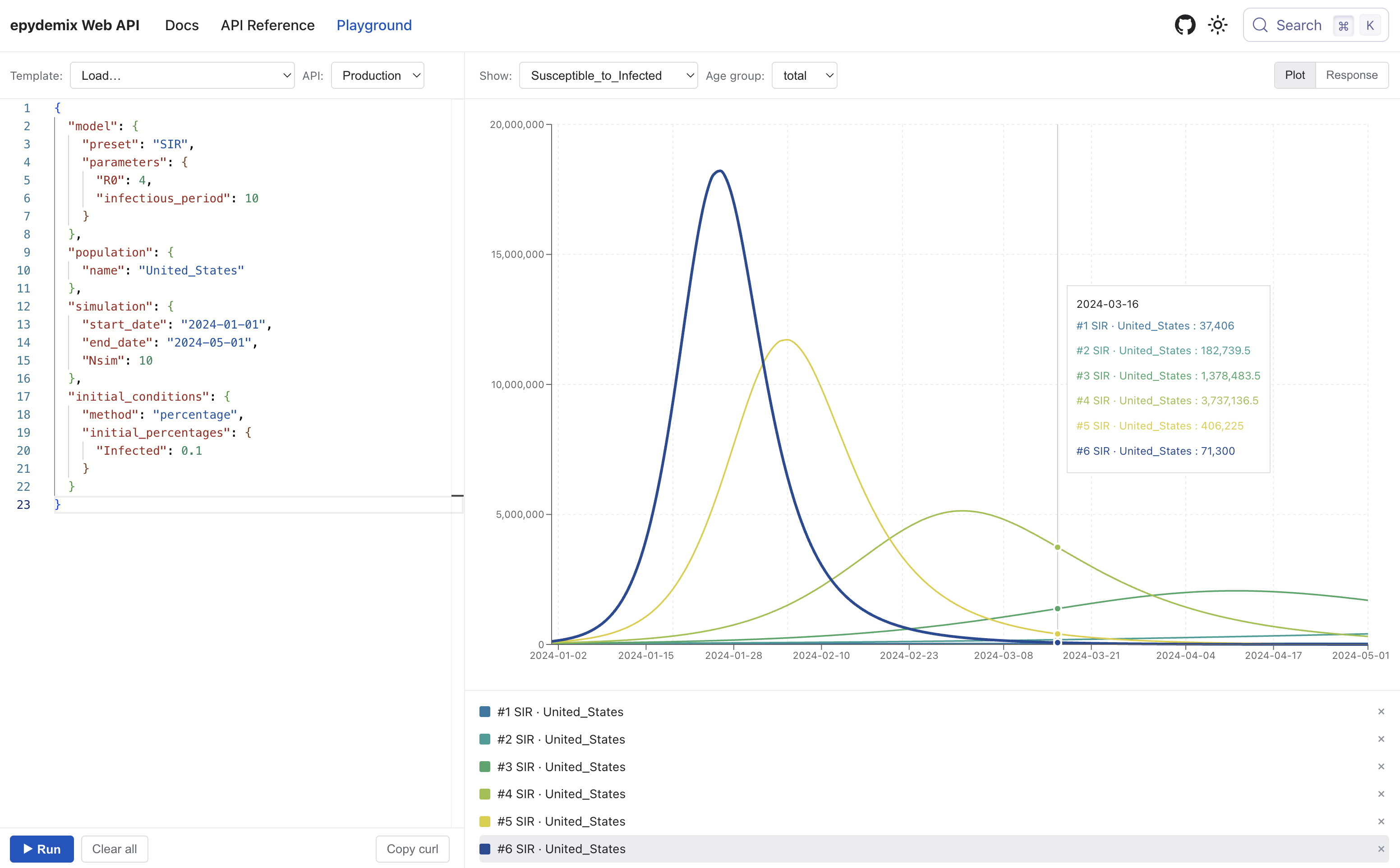
The [Playground](/playground) is an interactive page for testing the API directly from the browser.
## What you can do
- Write a simulation request in JSON or load one from preset templates
- Send the request to the API, and see the results in the preview pane
- View results as a time-series plot, switching compartments, transitions, age groups, and parameters
- Compare multiple runs (with different parameters or presets) by overlaying their plots
- Inspect and download the raw JSON response
- Copy the equivalent `curl` command to reproduce the request outside the playground
## When to use it
- Exploring the request shape before wiring up a client
- Iterating on parameters, dates, or `output` filters and seeing the effect immediately
- Sanity-checking a custom model or population against a known preset
- Confirming the effect of [parameter transformations](../model/parameter-transformations.mdx) such as seasonality, scaling, or overrides
## Open the playground
Click on [`Playground`](/playground) in the top navigation bar.
:::tip
For programmatic use, see [Running a Simulation](./running-a-simulation.mdx) for the full request and response shape, and the [API Reference](/api-reference) for an interactive request builder.
:::
---
# Custom Populations
Instead of a [preset](./presets.mdx), you can define a population inline by specifying age groups and contact matrices yourself. This is useful for synthetic populations (homogeneous mixing, toy two-group models) or for plugging in demographics and contact data that aren't available through epydemix.
To opt in, set `population.source` to `"custom"` and provide `age_groups` and `contact_matrices`.
## Structure
A custom population requires two things.
### Age groups
A mapping from group name to population count. **Insertion order matters**: it defines the row and column order used by every contact matrix and by any age-varying parameter.
```json
"age_groups": {
"A": 100000,
"B": 100000
}
```
### Contact matrices
One square matrix per layer, keyed by layer name. Each matrix must be `n` by `n` where `n = len(age_groups)`, and rows and columns follow the same order as `age_groups`. The keys define your layer set: pick names that match anything you'll target with [interventions](../running-a-simulation.mdx).
```json
"contact_matrices": {
"home": [[0.10, 0.05], [0.05, 0.10]],
"work": [[0.15, 0.20], [0.20, 0.15]]
}
```
The layer name `overall` is reserved by epydemix and rejected.
## Example: Homogeneous (single group)
The simplest case: one age group and a 1x1 contact matrix. This reproduces the classic homogeneous-mixing compartmental model.
```bash
curl -X POST BASE_URL/simulations \\
-H "Content-Type: application/json" \\
-d '{
"model": {
"preset": "SIR",
"parameters": {"transmission_rate": 0.3, "recovery_rate": 0.1}
},
"population": {
"source": "custom",
"name": "Homogeneous N=100k",
"age_groups": {"A": 100000},
"contact_matrices": {"all": [[1.0]]}
},
"simulation": {
"start_date": "2024-01-01",
"end_date": "2024-06-01",
"Nsim": 50
}
}'
```
## Example: Two age groups
A toy two-group population with a single mixing layer.
```bash
curl -X POST BASE_URL/simulations \\
-H "Content-Type: application/json" \\
-d '{
"model": {
"preset": "SIR",
"parameters": {"transmission_rate": 0.3, "recovery_rate": 0.1}
},
"population": {
"source": "custom",
"name": "Toy two-group",
"age_groups": {"A": 100, "B": 100},
"contact_matrices": {"all": [[0.2, 0.3], [0.3, 0.2]]}
},
"simulation": {
"start_date": "2024-01-01",
"end_date": "2024-01-31",
"Nsim": 5
}
}'
```
## Example: Multiple layers with an intervention
Custom layers can be targeted by interventions just like preset layers. Here a `lockdown` cuts contacts in the `work` layer to 50% for ten days.
```bash
curl -X POST BASE_URL/simulations \\
-H "Content-Type: application/json" \\
-d '{
"model": {
"preset": "SIR",
"parameters": {"transmission_rate": 0.3, "recovery_rate": 0.1}
},
"population": {
"source": "custom",
"name": "Two-layer custom",
"age_groups": {"A": 100, "B": 100},
"contact_matrices": {
"home": [[0.10, 0.05], [0.05, 0.10]],
"work": [[0.15, 0.20], [0.20, 0.15]]
}
},
"interventions": [
{
"layer_name": "work",
"start_date": "2024-01-10",
"end_date": "2024-01-20",
"reduction_factor": 0.5,
"name": "lockdown"
}
],
"simulation": {
"start_date": "2024-01-01",
"end_date": "2024-01-31",
"Nsim": 10
}
}'
```
## Validation rules
Requests that violate any of the following return `422`:
| Rule | What gets rejected |
|---|---|
| `age_groups` non-empty | `{}` |
| `contact_matrices` non-empty | `{}` |
| Each matrix is `n` by `n` where `n = len(age_groups)` | row count mismatch, non-square rows |
| Layer name is not `overall` | `{"overall": [[...]]}` |
---
# Overview
## What is a population?
A population defines **who is being simulated** and **how they mix**. Every simulation in epydemix is age-stratified, meaning that compartments and transitiosn are tracked separately for each age group, and the contact matrices control transmission between groups.
Specifically, a population provides:
- **Population demographics by age group**: named age bins with a population count each (e.g. `0-4`, `5-19`, `20-49`, `50-64`, `65+`).
- **Contact matrices by age group**: one square matrix per layer (`home`, `work`, `school`, `community`), where entry $(i, j)$ is the average number of contacts a person in group $i$ has with people in group $j$.
You can either pick a built-in [population preset](./presets.mdx) (real-world demographics and contact data for a specific country or subnational region, such as a US state) or define a [custom population](./custom-populations.mdx) inline.
## Contact Matrix
The contact matrix is what lets the model capture **heterogeneity of contacts across age groups**. In real data, the diagonal is typically the largest entry (people interact most with peers their own age, **assortative mixing**), and the strength varies by setting. The `school` layer is dominated by contacts among school-age groups, `work` is concentrated in working-age groups, and `home` mixes parents with children. Splitting contacts by layer makes this structure explicit, and lets [interventions](../running-a-simulation.mdx) target a single setting (e.g. closing schools) without touching the others.
A force of infection is computed by combining the contact matrices with the proportion of infectious individuals in each group, so age structure shapes both who gets infected first and the overall epidemic shape. Parameters like `transmission_rate` can also be specified per age group; see [Parameters](../model/parameters/overview.mdx).
## Example: Age-stratified SIR
Let's look at an example of how the contact matrix is used in actual epidemic models. The following is an deterministic ordinary differential equations for age-stratified SIR model, which is the mean-field equivalent of the stochastic simulation of our [SIR preset](../model/presets/sir.mdx). Note that the simulations in this API are fully **stochastic**: at each time step, transitions between compartments are drawn from binomial distributions, and `Nsim` independent runs are executed.
### Model
With age groups indexed by $i = 1, \dots, n$:
$$
\begin{aligned}
\frac{dS_i}{dt} &= -\lambda_i\, S_i \\
\frac{dI_i}{dt} &= \lambda_i\, S_i - \mu\, I_i \\
\frac{dR_i}{dt} &= \mu\, I_i
\end{aligned}
$$
with the per-group force of infection
$$
\lambda_i = \beta \sum_{j=1}^{n} C_{ij}\, \frac{I_j}{N_j}.
$$
$S_i, I_i, R_i$ are the compartment counts in age group $i$, $N_i = S_i + I_i + R_i$ is the group size, $\beta$ is `transmission_rate`, $\mu$ is `recovery_rate`, and $C_{ij}$ is the average number of contacts a person in group $i$ has with people in group $j$, summed across the contact layers (`home`, `work`, `school`, `community`).
The same pattern applies to any model: every compartment becomes a vector indexed by age group, and any mediated transition uses the contact matrix in its force-of-infection term. SEIR, SIS, and custom models with extra compartments all follow this structure.
### Calibrating $\beta$ from $R_0$
In the homogeneous (single-group) case, $R_0 = \beta / \mu$. With age stratification, the contact matrix takes over the role of "average contacts per person" and the relation becomes
$$
R_0 = \frac{\beta}{\mu}\, \rho(C),
\qquad \text{equivalently} \qquad
\beta = \frac{R_0\, \mu}{\rho(C)},
$$
where $\rho(C)$ is the **spectral radius (largest eigenvalue) of the overall contact matrix** (the sum of the layer matrices). The spectral radius is returned as `spectral_radius.overall` by [`GET /populations/{name}/contacts`](./presets.mdx#get-contact-matrices), so you can plug it straight in to pick a `transmission_rate` that targets a desired $R_0$.
To do this calculation directly inside the request, use the reserved name `CONTACT_MATRIX_EIGENVALUE_ALL` (= $\rho(C)$) from a [calculated parameter](../model/parameters/overview.mdx#calculated-parameters):
```json
{
"parameters": {
"R0": 1.5,
"gamma": 0.1,
"recovery_rate": "gamma",
"transmission_rate": "R0 * gamma / CONTACT_MATRIX_EIGENVALUE_ALL"
}
}
```
---
# Population Presets
Population presets are built-in populations published in the [epydemix-data](https://github.com/epistorm/epydemix-data) repository. Each preset comes with age-distribution data and one or more contact-matrix sources, ready to use without you having to provide demographic data yourself. It lets you simulate epidemic for specific location and population, reflecting the demographics and contact structure.
For background on what a population is and how the contact matrix shapes an age-stratified simulation, see [Overview](./overview.mdx).
## List all populations
Browse every population available in the API along with its supported contact sources.
API reference: [`GET /api/v1/populations`](/api-reference).
```bash
curl BASE_URL/populations
```
Example response (truncated):
```json
{
"populations": [
{
"name": "Afghanistan",
"display_name": "Afghanistan",
"total_population": 42044654,
"available_contact_sources": ["prem_2021"]
},
{
"name": "United_States",
"display_name": "United States",
"total_population": 338120586,
"available_contact_sources": ["mistry_2021"]
}
],
"total": 461
}
```
### Subnational populations
Beyond country-level entries, the API also exposes **subnational regions** (states, provinces, prefectures) using the naming convention `Country__Region` (double underscore between country and region). They behave exactly like country populations: pass the full identifier as `name` to any populations endpoint or as `population.name` in a simulation.
| Country | Subdivisions | Example identifier |
|---|---|---|
| United States | 50 states + DC (plus ~3,100 counties; see below) | `United_States__Massachusetts`, `United_States__California`, `United_States__Texas` |
| Russia | 83 | `Russia__Moscow`, `Russia__St._Petersburg` |
| Japan | 47 prefectures | `Japan__Tokyo-to`, `Japan__Osaka-fu`, `Japan__Aichi-ken` |
| India | 32 | `India__Maharashtra`, `India__Karnataka` |
| China | 31 | `China__Beijing`, `China__Guangdong` |
| Canada | 13 provinces/territories | `Canada__Ontario`, `Canada__Quebec` |
| South Africa | 9 | `South_Africa__Gauteng`, `South_Africa__Western_Cape` |
| Australia | 8 states/territories | `Australia__Victoria`, `Australia__New_South_Wales` |
Use [`GET /api/v1/populations`](/api-reference) to enumerate every available identifier.
Example: simulate an outbreak in Massachusetts.
```bash
curl -X POST BASE_URL/simulations \\
-H "Content-Type: application/json" \\
-d '{
"model": {"preset": "SIR", "parameters": {"transmission_rate": 0.3, "recovery_rate": 0.1}},
"population": {"name": "United_States__Massachusetts"},
"simulation": {"start_date": "2024-01-01", "end_date": "2024-06-01", "Nsim": 50}
}'
```
:::note
All subnational entries currently ship only the `mistry_2021` contact source, so the `prem_2017` / `prem_2021` overrides available on most country populations don't apply here.
:::
### United States county-level
The US is further divided into ~3,100 **counties**. Demographic distributions are sourced from the US Census Bureau (2023); contact matrices are inherited from the corresponding state (in the absence of county-specific survey data). Identifiers follow the same convention with one more level: `United_States____`.
| Example | Description |
|---|---|
| `United_States__Massachusetts__Suffolk_County` | Boston and surrounding cities |
| `United_States__New_York__Kings_County` | Brooklyn |
| `United_States__California__Los_Angeles_County` | Los Angeles |
```bash
curl -X POST BASE_URL/simulations \\
-H "Content-Type: application/json" \\
-d '{
"model": {"preset": "SIR", "parameters": {"transmission_rate": 0.3, "recovery_rate": 0.1}},
"population": {"name": "United_States__Massachusetts__Suffolk_County"},
"simulation": {"start_date": "2024-01-01", "end_date": "2024-06-01", "Nsim": 50}
}'
```
## Inspect a population
Look up demographic details for a single population: total size, age groups, and which contact sources and layers it ships with.
API reference: [`GET /api/v1/populations/{name}`](/api-reference).
```bash
curl BASE_URL/populations/United_States
```
Returns the total population, the default 5-group age aggregation, the raw per-single-year age distribution, available contact sources, and contact layers.
Example response (`age_distribution` truncated):
```json
{
"name": "United_States",
"display_name": "United States",
"total_population": 338120586,
"age_groups": {
"0-4": 18608139,
"5-19": 63540783,
"20-49": 132780169,
"50-64": 63172279,
"65+": 60019216
},
"age_distribution": {
"0": 3667336,
"1": 3713583,
"2": 3630098,
"...": 0,
"83": 1221647,
"84+": 7418335
},
"contact_sources": ["mistry_2021"],
"default_contact_source": "mistry_2021",
"available_layers": ["school", "work", "home", "community"]
}
```
## Get contact matrices
Fetch the per-layer mixing matrices used to compute the force of infection between age groups.
API reference: [`GET /api/v1/populations/{name}/contacts`](/api-reference).
```bash
curl BASE_URL/populations/United_States/contacts
```
Returns one matrix per layer (`home`, `work`, `school`, `community`), the combined `overall` matrix, and the spectral radius of each. Pass `?contacts_source=prem_2021` or `?layers=home&layers=work` to narrow the response.
Example response (matrix entries rounded to two decimals for brevity):
```json
{
"population_name": "United_States",
"contact_source": "default",
"age_groups": ["0-4", "5-19", "20-49", "50-64", "65+"],
"layers": {
"school": [
[0.68, 1.27, 0.19, 0.09, 0.01],
[0.41, 8.82, 1.08, 0.29, 0.04],
[0.03, 0.53, 1.01, 0.09, 0.02],
[0.03, 0.30, 0.17, 0.04, 0.01],
[0.01, 0.07, 0.07, 0.01, 0.00]
],
"work": [
[0.00, 0.00, 0.00, 0.00, 0.00],
[0.00, 0.01, 0.23, 0.10, 0.01],
[0.00, 0.11, 3.31, 1.40, 0.14],
[0.00, 0.09, 2.86, 1.23, 0.12],
[0.00, 0.01, 0.44, 0.19, 0.02]
],
"home": [["..."]],
"community": [["..."]]
},
"overall": [
[1.42, 2.68, 3.79, 0.81, 0.43],
[0.87, 10.61, 4.50, 1.39, 0.50],
[0.64, 2.23, 7.17, 2.47, 0.66],
[0.28, 1.40, 5.06, 3.44, 0.92],
[0.22, 0.79, 2.10, 1.34, 2.17]
],
"spectral_radius": {
"school": 8.96,
"work": 4.55,
"home": 3.75,
"community": 2.79,
"overall": 14.04
}
}
```
Each row of `overall` corresponds to the same age group as `age_groups[i]`; the matrix is the sum of the per-layer matrices and is what the simulation uses by default. The diagonal of the `school` layer is dominated by the `5-19` entry (8.82), illustrating the assortative mixing discussed in the [Overview](./overview.mdx#contact-matrix).
### Contact sources
Three sources are available for most countries:
| Source | Description |
|---|---|
| `prem_2017` | Prem et al. 2017 synthetic matrices |
| `prem_2021` | Prem et al. 2021 update |
| `mistry_2021` | Mistry et al. 2021 (default for most populations) |
## Using population in a simulation
### Population by name
The minimal form to use population in simulations is by setting `population.name`. The default contact source is used and the default 5-group aggregation is applied.
API reference: [`POST /api/v1/simulations`](/api-reference).
```bash
curl -X POST BASE_URL/simulations \\
-H "Content-Type: application/json" \\
-d '{
"model": {"preset": "SIR", "parameters": {"transmission_rate": 0.3, "recovery_rate": 0.1}},
"population": {"name": "United_States"},
"simulation": {"start_date": "2024-01-01", "end_date": "2024-06-01", "Nsim": 50}
}'
```
### Pick a contact source and layers
Override the defaults to choose which contact dataset is loaded and which layers it includes.
```bash
curl -X POST BASE_URL/simulations \\
-H "Content-Type: application/json" \\
-d '{
"model": {"preset": "SIR", "parameters": {"transmission_rate": 0.3, "recovery_rate": 0.1}},
"population": {
"name": "United_States",
"contacts_source": "prem_2021",
"layers": ["home", "work", "school", "community"]
},
"simulation": {"start_date": "2024-01-01", "end_date": "2024-06-01", "Nsim": 10}
}'
```
Omitting `layers` includes every layer the source provides.
### Custom age-group aggregation
By default, populations are returned in the 5-group `mistry_2021`/`prem_2021` aggregation. Use `age_group_mapping` to merge the source single-year groups into your own bins. Keys are your new group names; values list the source groups to merge.
```bash
curl -X POST BASE_URL/simulations \\
-H "Content-Type: application/json" \\
-d '{
"model": {"preset": "SIR", "parameters": {"transmission_rate": 0.3, "recovery_rate": 0.1}},
"population": {
"name": "United_States",
"contacts_source": "prem_2021",
"age_group_mapping": {
"0-4": ["0-4"],
"5-17": ["5-9", "10-14", "15-19"],
"18-49": ["20-24", "25-29", "30-34", "35-39", "40-44", "45-49"],
"50-64": ["50-54", "55-59", "60-64"],
"65+": ["65-69", "70-74", "75+"]
}
},
"simulation": {"start_date": "2024-01-01", "end_date": "2024-12-31", "Nsim": 10}
}'
```
The resolved age groups become the row/column order of contact matrices and the index for any age-varying parameters in `model.parameters`.
:::info
Population data comes from the [epydemix-data](https://github.com/epistorm/epydemix-data) repository, which lists every available country and the source datasets behind each contact matrix.
:::
---
# Running a Simulation
This guide walks through running your first simulation using the SIR model with US population data.
## 1. Check available populations
```bash
curl BASE_URL/populations
```
Pick a population name from the list. We'll use `United_States`. See [Population Presets](./populations/presets.mdx) for the full set of options (contact sources, layers, age-group remapping) and [Custom Populations](./populations/custom-populations.mdx) for inline age groups and contact matrices.
## 2. Check available presets
```bash
curl BASE_URL/models/presets
```
We'll use the `SIR` preset. See [Model Presets](./model/presets/overview.mdx) for the SIR / SEIR / SIS / V-SEIHR compartments and default parameters, or [Custom Models](./model/custom-models.mdx) to define your own compartments and transitions.
## 3. Send a simulation request
```bash
curl -X POST BASE_URL/simulations \\
-H "Content-Type: application/json" \\
-d '{
"model": {
"preset": "SIR",
"parameters": {
"transmission_rate": 0.3,
"recovery_rate": 0.1
}
},
"population": {
"name": "United_States"
},
"simulation": {
"start_date": "2024-01-01",
"end_date": "2024-06-01",
"Nsim": 10
},
"initial_conditions": {
"method": "percentage",
"initial_percentages": {"Infected": 0.1}
}
}'
```
The `initial_conditions` block seeds the compartments at the start of the simulation. Here, 0.1% of the population is placed in `Infected` and the rest in `Susceptible`. Omit the block entirely and ~0.05% of each age group is seeded as `Infected` by default; switch `method` to `"absolute"` to set exact per-age counts. See [Initial Conditions](./initial-conditions.mdx) for the full reference.
## 4. Read the response
The response contains `metadata`, `results`, and a `status` field. By default the API returns everything: all compartments and transitions, all age groups (plus `total`), all seven standard quantiles, and a `summary` with peaks and cumulative totals per age group. You can narrow any of these via `output` (see [Customizing output](#5-customizing-output)).
```json
{
"simulation_id": "sim_c9617343b215",
"status": "completed",
"metadata": {
"model": {
"preset": "SIR",
"compartments": ["Susceptible", "Infected", "Recovered"]
},
"population": {
"name": "United_States",
"contacts_source": "mistry_2021",
"layers": ["home", "work", "school", "community"],
"age_group_mapping": null,
"total": 338120586,
"age_groups": {
"0-4": 18608139,
"5-19": 63540783,
"20-49": 132780169,
"50-64": 63172279,
"65+": 60019216
}
},
"simulation": {
"start_date": "2024-01-01",
"end_date": "2024-06-01",
"Nsim": 10,
"dt": 1.0,
"seed": null,
"resample_frequency": "D"
}
},
"results": {
"compartments": {
"dates": ["2024-01-01", "2024-01-02", "..."],
"data": {
"Susceptible": {
"total": {
"0.5": [337330136.0, 334286966.0, "..."],
"0.025": [337330089.45, 334285584.7, "..."],
"0.975": [337330182.55, 334288347.3, "..."]
}
}
}
},
"transitions": {
"dates": ["2024-01-01", "2024-01-02", "..."],
"data": {
"Susceptible_to_Infected": {
"total": {
"0.5": [621391.0, 3043170.0, "..."],
"0.025": [621344.45, 3041835.25, "..."],
"0.975": [621437.55, 3044504.75, "..."]
}
}
}
},
"summary": {
"peaks": {
"Infected": {
"total": {
"quantiles": {
"0.025": 121800000.0,
"0.5": 124500000.0,
"0.975": 127100000.0
},
"peak_date": "2024-02-14"
},
"0-4": { "quantiles": { "0.5": 4120000.0, "...": 0 }, "peak_date": "2024-02-13" },
"65+": { "quantiles": { "0.5": 16800000.0, "...": 0 }, "peak_date": "2024-02-16" }
}
},
"totals": {
"Susceptible_to_Infected": {
"total": { "quantiles": { "0.025": 213000000.0, "0.5": 215000000.0, "0.975": 217000000.0 } },
"0-4": { "quantiles": { "0.5": 11800000.0, "...": 0 } }
}
}
}
}
}
```
Results are organized as quantiles (median, confidence intervals) across simulation runs. Both `compartments` and `transitions` follow the same nested structure: `name -> age_group -> quantile -> [values]`. The `total` age group is the sum across all age groups.
`summary` mirrors that shape without the time dimension. `peaks` is `compartment -> age_group -> {quantiles, peak_date}` and carries the maximum value reached during the simulation window per quantile. `totals` is `transition -> age_group -> {quantiles}` and carries the cumulative number of transition events over the whole window.
## 5. Customizing output
Everything under `output` is optional; sensible defaults cover most cases. You can narrow the response with any combination of:
```json
{
"output": {
"quantiles": [0.1, 0.5, 0.9],
"age_groups": ["total"],
"compartments": ["Infected"],
"transitions": ["Susceptible_to_Infected"],
"summary": {
"peak_compartments": ["Infected"],
"total_transitions": []
}
}
}
```
- `quantiles` drives both the trajectory quantiles and the `summary` quantiles.
- `age_groups` filters both the trajectory age groups and the `summary` age groups. Use `["total"]` to skip the per-age breakdown entirely.
- `compartments` / `transitions` filter the trajectory section only.
- `summary.peak_compartments` / `summary.total_transitions`: omit to include every compartment / transition; pass `[]` to explicitly opt out of that half of the summary. An empty array for both leaves `summary: null`.
## 6. Increase Nsim for production use
Start with `Nsim: 10` while testing, then increase to 100 or more for reliable estimates.
## 7. One-liner example
For a quick read of one stat from the response, pipe through [`jq`](https://jqlang.org/). For example, the median peak of `Infected` summed across all age groups along with its date:
```bash
curl -s -X POST BASE_URL/simulations \\
-H "Content-Type: application/json" \\
-d '{
"model": {"preset": "SIR", "parameters": {"transmission_rate": 0.3, "recovery_rate": 0.1}},
"population": {"name": "United_States"},
"simulation": {"start_date": "2024-01-01", "end_date": "2024-06-01", "Nsim": 100}
}' | jq '.results.summary.peaks.Infected.total | {peak_date, median: .quantiles["0.5"]}'
```
```json
{
"peak_date": "2024-01-06",
"median": 290283372.5
}
```
:::tip
Use the [API Reference](/api-reference) to build and send requests interactively without writing curl commands.
:::
## Next
Try the same request in the [Playground](./playground.mdx) to iterate on parameters and see plots without leaving the browser.
---
# Campaigns
This page covers the per-campaign fields and rollout strategies inside the `vaccination` block. For the surrounding block structure and `flows` configuration, see the [Overview](./overview.mdx).
## Quick start
The fastest path is using the `V-SEIHR` model preset with a flat-count vaccination campaign. In the following example, we roll out vaccination starting in February 2025 with a target of 100,000 doses per day held constant across the window. See [Dose allocation](./overview.mdx#dose-allocation) for how the daily dose count splits across age groups.
```bash
curl -X POST BASE_URL/simulations \\
-H "Content-Type: application/json" \\
-d '{
"model": {
"preset": "V-SEIHR",
"parameters": {
"R0": 2.5,
"incubation_period": 3.0,
"infectious_period": 2.5,
"hosp_duration": 5.0,
"hosp_proportion": 0.05,
"VE_S": 0.7,
"VE_H": 0.85
}
},
"population": {"name": "United_States"},
"simulation": {"start_date": "2025-01-01", "end_date": "2025-06-30", "Nsim": 10},
"vaccination": {
"campaigns": [
{
"start_date": "2025-02-01",
"end_date": "2025-04-30",
"rollout": {"type": "flat_count", "daily_doses": 100000}
}
]
}
}'
```
The response includes the resulting `Susceptible_to_Susceptible_vax` transition series; see [Inspecting the rollout](./overview.mdx#inspecting-the-rollout) for what to look at.
## Campaign fields
Each entry in `campaigns` describes one rollout:
| Field | Required | Description |
|---|---|---|
| `name` | no | Free-text label echoed back in `metadata.vaccination`. Handy for keeping multiple overlapping campaigns straight. |
| `start_date` | yes | Campaign start (`YYYY-MM-DD`), inclusive. |
| `end_date` | yes | Campaign end (`YYYY-MM-DD`), inclusive. Must be `≥ start_date`. |
| `rollout` | yes | Rollout strategy. v1 supports `flat_count`; the `type` field is the discriminator. See [Rollout strategies](#rollout-strategies). |
| `target_age_groups` | no | List of age-group labels (e.g. `["50-64", "65+"]`). Must be unique and must match labels from the resolved population. `null` (the default) means all groups. |
## Rollout strategies
### Flat rollout (count)
A constant `daily_doses` count is scheduled every day across the campaign window, distributed proportionally to the source-compartment population in each targeted age group.
"Flat" refers to the *scheduled* budget, not the *delivered* curve: as the source pool depletes (through vaccination, infections, etc.), the actual daily delivered count can drift below `daily_doses`. If the live pool drops below `daily_doses` per step, the per-source stochastic draw saturates against the available population; if the pool is empty, no doses are delivered that step. See the [Dose allocation](./overview.mdx#dose-allocation) section for the per-step competing-risks draw.
| Field | Required | Description |
|---|---|---|
| `type` | yes | Literal `"flat_count"`. The discriminator. |
| `daily_doses` | yes | Target doses delivered per day. Must be `> 0`. |
Example
Here is an example of V-SEIHR model run on a 1,000,000 homogeneous population ($R_0 = 1.4$, $\mathrm{VE}_S = 0.85$, $\mathrm{VE}_H = 0.9$, 0.02% initial infections, no waning), with a single campaign scheduled at 5,000 doses/day from Feb 1 to Oct 15, 2025 (100 stochastic runs, median plotted).
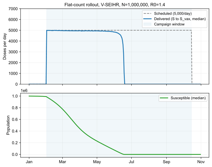
The scheduled budget (dashed) holds at 5,000/day across the entire window, but the delivered count drops to zero around the end of May as $S$ is exhausted by the epidemic plus vaccination.
## Custom-model usage
You can define a custom model that incorporates the effects of vaccination and takes advantage of the `vaccination` block. What you need is a model whose compartments include both a source and a vaccinated target, and (typically) a vaccinated layer that mirrors the unvaccinated transitions with vaccine-efficacy-attenuated rates. The block then drives doses across the `source → target` pairs declared in `flows`. You can model the effects of vaccination through transformed parameters (e.g. severity reduction) and additional transitions.
On a custom model the `flows` field is **required**; there is no default. Every `source` and (non-null) `target` must reference a compartment declared in `model.compartments`.
```bash
curl -X POST BASE_URL/simulations \\
-H "Content-Type: application/json" \\
-d '{
"model": {
"compartments": ["S", "V", "I", "R"],
"parameters": {
"transmission_rate": 0.3,
"transmission_rate_v": "(1 - VE_S) * transmission_rate",
"VE_S": 0.7,
"recovery_rate": 0.1
},
"transitions": [
{"source": "S", "target": "I", "kind": "mediated", "params": ["transmission_rate", "I"]},
{"source": "V", "target": "I", "kind": "mediated", "params": ["transmission_rate_v", "I"]},
{"source": "I", "target": "R", "kind": "spontaneous", "params": ["recovery_rate"]}
]
},
"population": {"name": "Italy"},
"simulation": {"start_date": "2025-01-01", "end_date": "2025-06-30", "Nsim": 10},
"vaccination": {
"flows": [{"source": "S", "target": "V"}],
"campaigns": [
{
"start_date": "2025-02-01",
"end_date": "2025-03-31",
"rollout": {"type": "flat_count", "daily_doses": 50000}
}
]
}
}'
```
## Multiple campaigns
Listing more than one campaign lets you stack rollouts. Two overlapping `flat_count` campaigns add their daily doses at every step. Use this for booster waves, prioritization changes (e.g. open eligibility on a given date by adding a younger-age campaign mid-rollout), or to compare a baseline campaign against an accelerated counterfactual.
```bash
curl -X POST BASE_URL/simulations \\
-H "Content-Type: application/json" \\
-d '{
"model": {
"preset": "V-SEIHR",
"parameters": {"R0": 2.5, "VE_S": 0.7, "VE_H": 0.85}
},
"population": {
"name": "United_States",
"contacts_source": "prem_2021",
"age_group_mapping": {
"0-17": ["0-4", "5-9", "10-14", "15-19"],
"18-49": ["20-24", "25-29", "30-34", "35-39", "40-44", "45-49"],
"50-64": ["50-54", "55-59", "60-64"],
"65+": ["65-69", "70-74", "75+"]
}
},
"simulation": {"start_date": "2025-01-01", "end_date": "2025-06-30", "Nsim": 10},
"vaccination": {
"campaigns": [
{
"name": "phase 1 (older adults)",
"start_date": "2025-02-01",
"end_date": "2025-03-31",
"target_age_groups": ["65+"],
"rollout": {"type": "flat_count", "daily_doses": 40000}
},
{
"name": "phase 2 (open eligibility)",
"start_date": "2025-03-15",
"end_date": "2025-05-31",
"target_age_groups": ["18-49", "50-64", "65+"],
"rollout": {"type": "flat_count", "daily_doses": 80000}
}
]
}
}'
```
---
# Overview
Vaccination moves individuals between compartments: a **donor pool** (typically `Susceptible`) and a **vaccinated counterpart** (typically `Susceptible_vax`), in the age groups a campaign targets and during its time window. Protection comes from the vaccinated layer using attenuated parameters (lower susceptibility, lower severity, etc.).
## Quick start
The `vaccination` block of the API request only defines the rollout (e.g., schedule, doses, targets, flows), and the actual effects from vaccination are modeled with [`parameters` from the `model` block](../model/parameters/overview.mdx).
The [`V-SEIHR` model preset](../model/presets/v-seihr.mdx) is one of the examples which uses vaccination feature, where we have vaccinated branch of compartments with `VE_S` and `VE_H` efficacy parameters. In this preset, vaccination by default generates the flow `Susceptible → Susceptible_vax`.
```json5
{
"model": {
"preset": "V-SEIHR",
"parameters": {
"R0": 2.5,
"incubation_period": 3.0,
"infectious_period": 2.5,
"hosp_duration": 5.0,
"hosp_proportion": 0.05,
"VE_S": 0.7, // vaccine efficacy against infection
"VE_H": 0.85
}
},
"population": {"name": "United_States"},
"simulation": {"start_date": "2025-01-01", "end_date": "2025-06-30", "Nsim": 10},
"vaccination": {
// "flows" is optional on V-SEIHR (defaults to S → S_vax pair); set it to override.
// "flows": [{"source": "Susceptible", "target": "Susceptible_vax"}],
"campaigns": [
{
"start_date": "2025-02-01",
"end_date": "2025-04-30",
"rollout": {"type": "flat_count", "daily_doses": 100000}
}
]
}
}
```
## `vaccination` block
The block declares which compartments are involved in the rollout (`flows`) and which campaigns drive doses (`campaigns`). On `V-SEIHR` the default flow is `Susceptible → Susceptible_vax`; custom models must declare flows explicitly.
| Field | Required | Description |
|---|---|---|
| `flows` | for custom models | List of `{source, target}` compartment pairs. V-SEIHR defaults to `Susceptible → Susceptible_vax`. See [Flows](#flows) for shapes (including dose sinks) and validation. |
| `campaigns` | yes (≥1) | List of campaigns, each with its own dates, target age groups, and dose schedule. Multiple campaigns may overlap and their per-step dose schedules add. See [Campaigns](./campaigns.mdx) for the per-campaign fields and rollout strategies. |
## From doses to a per-individual rate
### Rate calculation
Each campaign turns a daily **dose budget** $d_c(t)$ into a per-individual vaccination rate $r_c(t)$ by spreading those doses across the **live eligible pool**:
$$
r_c(t) = \frac{d_c(t)}{\displaystyle\sum_{X \in \mathcal{S}}\;\sum_{j \in \mathcal{A}_c} X_j(t)}.
$$
Here $\mathcal{A}_c$ is the set of age groups campaign $c$ targets, $\mathcal{S}$ is the set of source compartments configured in `flows`, and $X_j(t)$ is the live count in source $X$ and age group $j$ at step $t$. The denominator is recomputed every step, so it tracks the pool as people leave or re-enter. In the simplest case (a single `Susceptible → Susceptible_vax` flow), it collapses to "daily doses divided by live susceptibles".
### Flows
`flows` is a list of `{source, target}` pairs naming which compartments compete for doses and where vaccinated individuals move to. Every `source` contributes to the rate denominator above, and every flow with a non-null `target` emits a `source → target` transition. Entries with `target: null` are **dose sinks**: they shrink the rate denominator without moving anyone, useful when real campaigns can't pre-screen recipients (doses landing on already-recovered people are still consumed).
A few common shapes:
```json5
// 1. Perfect targeting (V-SEIHR default).
"flows": [{"source": "Susceptible", "target": "Susceptible_vax"}]
// 2. Dose sink: S + R compete for doses but only S transitions.
// Models a real-world campaign that cannot pre-screen recipients.
"flows": [
{"source": "Susceptible", "target": "Susceptible_vax"},
{"source": "Recovered", "target": null}
]
// 3. Multi-target: one budget shared across two susceptible strata.
// Each source draws from the shared budget in proportion to its live size,
// and each pair emits its own `_to_` transition at the same
// per-individual rate.
"flows": [
{"source": "Susceptible", "target": "Susceptible_vax"},
{"source": "Susceptible_2", "target": "Susceptible_2_vax"}
]
```
For example with shape #2: 4,000 susceptibles and 56,000 recovered sharing 1,000 daily doses yield an expected `S → S_vax` count of $1{,}000 \times 4{,}000 / 60{,}000 \approx 67$; the rest are absorbed by `R`.
## Dose allocation
The per-individual rate is **shared** across all targeted groups and sources, so each (source, group) cell receives doses in proportion to its live population. With a single flow `[{S, S_vax}]`, a `flat_count` campaign targeting two age groups holding 4,000 and 6,000 susceptibles and a 1,000-dose-per-day budget delivers 400 and 600 doses respectively (in expectation).
At each step the simulator updates each source compartment independently with a multinomial draw over all of its out-edges. Every active vaccination flow leaving $X$ contributes the campaign rate $r_c(t)$ from above, alongside any non-vaccination rates $q^{X,k}_i(t)$ on the same source (e.g. infection $S \to E$).
Bundling them into the total per-individual out-rate
$$
H_i^{X}(t) \;=\; \underbrace{\sum_{c\,:\,i \in \mathcal{A}_c,\,X \in \mathcal{S}_c} r_c(t)}_{\text{vaccination}} \;+\; \underbrace{\sum_{k} q^{X,k}_i(t)}_{\text{other out-edges}},
$$
the per-step counts out of $X_i$ are sampled jointly as
$$
\bigl(\Delta_{\text{stay},i},\ \Delta_{Z_1,i},\ \Delta_{Z_2,i},\ \ldots\bigr) \;\sim\; \mathrm{Multinomial}\bigl(X_i(t),\ \mathbf{p}_i\bigr),
$$
where $\{Z_k\}$ enumerates the destinations reachable from $X$ (the vaccination target $Y$ is one of them) and $\mathbf{p}_i$ splits the total leave probability $1 - e^{-H_i^{X}\,dt}$ among them in proportion to each edge's rate.
In expectation, $Y$ thus receives
$$
\mathbb{E}[\Delta Y_i(t)] \;\approx\; r_c(t)\,X_i(t)\,dt,
$$
If vaccination is the only out-edge of $X_i$, the multinomial draw reduces to a binomial draw.
## Vaccine efficacy
How much protection vaccination confers is a property of the **model**, not the rollout block. The [`V-SEIHR` preset](../model/presets/v-seihr.mdx#vaccine-efficacy) defines `VE_S` (against infection) and `VE_H` (against hospitalization); see the preset page for how they enter the dynamics. Custom models can mirror the same pattern with their own efficacy expressions.
## Inspecting the rollout
Each transitioning flow surfaces as a regular transition in the response. For the default V-SEIHR rollout, look for `Susceptible_to_Susceptible_vax` under `results.transitions.data`. Note that flows with dose sinks (`target: null`) emit no transition.
The request itself is echoed back under `metadata.vaccination`, including the resolved `flows` list.
:::tip
Use the [API Reference](/api-reference) to explore the vaccination schema field-by-field and try requests interactively.
:::
---
# Introduction
epydemix Web API is a REST API for running epidemic simulations powered by [epydemix](https://github.com/epistorm/epydemix).
## Overview
The API exposes epydemix's simulation engine over HTTP. You can run compartmental models (SIR, SEIR, SIS) against built-in population data by sending a single JSON request. No Python environment required on the client side.
## How it works
1. Pick a model preset and population
2. POST a simulation request with your parameters
3. Get back compartment trajectories for each simulation run
## Endpoints
| Method | Path | Description |
|--------|------|-------------|
| POST | [`/api/v1/simulations`](/api-reference) | Run a simulation |
| GET | [`/api/v1/populations`](/api-reference) | List available populations |
| GET | [`/api/v1/populations/{name}`](/api-reference) | Get population details |
| GET | [`/api/v1/populations/{name}/contacts`](/api-reference) | Get contact matrices |
| GET | [`/api/v1/models/presets`](/api-reference) | List model presets |
| GET | [`/api/v1/health`](/api-reference) | Health check |
The [API Reference](/api-reference) has interactive docs where you can explore schemas and send requests directly.
---
# Configuration
The API reads configuration from environment variables.
| Variable | Default | Description |
|----------|---------|-------------|
| `APP_NAME` | `epydemix WebAPI` | Application name shown in API docs |
| `APP_VERSION` | `0.1.1` | API version |
| `API_V1_PREFIX` | `/api/v1` | URL prefix for all v1 endpoints |
| `WARM_CACHE_ON_STARTUP` | `false` | Pre-load population data at startup |
| `WARM_CACHE_POPULATIONS` | `[]` | List of population names to pre-load |
## Cache warming
Population data is loaded on first request by default. Setting `WARM_CACHE_ON_STARTUP=true` pre-loads specified populations at startup, which reduces latency on the first request for those populations.
```bash
WARM_CACHE_ON_STARTUP=true
WARM_CACHE_POPULATIONS=["United_States", "Italy"]
```
---